Introduction

The Okavango Delta is a flood-pulse driven mosaic of patchy woodlands, permanent swamps, and seasonally flooded grasslands that lie within the otherwise dry and sandy Kalahari Basin. It is the world’s largest inland delta, with a catchment area that can easily be seen from space (Figure 1). The delta’s floodwaters are originating from the Angolan highlands, where water is channeled through the Cuito and Cubango rivers into the Okavango river. The Okavango river eventually splits into many different channels that inundate a massive alluvial fan, covering an area between 5’000 and 15’000 km^2. Because of the shallow gradient of the delta (1/5600 at the upper floodplains and 1/3400 at the lower floodplains) water only slowly descends from the catchment areas in Angola into the Okavango Delta. As a result, the flood reaches its prime extent during the peak dry season (in July or August), when local rains have long ceased. The massive inflow of fresh-water during this otherwise dry period allows many species to survive in this arid ecosystem and attracts massive herds of elephants and antelopes, turning the Delta into a thriving hotspot of biodiversity.

Figure 1: Satellite image of Southern Africa. The Okavango Delta is clearly visible due to its dark green hue. The delta is fed by water that is collected in catchment areas in the Angolan highlands and only slowly descends thorugh the Delta’s tributaries. In fact, the flood takes so long to arrive that it reaches the distal ends of the delta during the peak dry season.

The Okavango Delta’s flood extent is highly dynamic and drastically changes across and within years (Figure 2). Being able to depict flood extents during different points in time is therefore vital to better understand species behavior and movement patterns. Thanks to data from numerous freely accessible satellites, remote sensing opens up new avenues for rendering flood patterns of the Okavango Delta at unprecedented spatio-temporal scales. Historically, spatial ecologists have utilized normalized differences indices (NDs) to remote sense various properties of a landscape from satellite imagery. With respect to remote sensing surface water, the normalized difference in water index (NDWI) has proven particularly useful. However, the Okavango Delta is a more tricky case, as areas inundated by water are often not recognizable as such. The main reason for this is that the delta’s floodwaters are incredibly shallow, such that water is often obstructed by vegetation (e.g., tall grass). In this situation, the NDWI tends to underestimate the true extent of the delta’s flood.

Figure 2: Satellite images of the Okavango Delta during the dry season (but peak flood) versus its extent during the wet season (but low flood).

To address this shortcoming, the Okavango Delta Research Institute has developed a remote sensing algorithm that is specifically tailored towards detecting flooded areas across the Okavango Delta. The algorithm utilizes MODIS MCD43A4 satellite data, which provides updated composite imagery on an 8 daily basis. Thanks to MODIS’ high revisitation rate, these 8 daily composites are almost guaranteed to be cloud-free, thus providing a near-continuous monitoring of the Delta. This comes at the cost of a relatively coarse spatial resolution of 500 m. Nevertheless, 500 m will suffice for most ecological applications.

I have repeatedly applied the algorithm developed by ORI to obtain flood maps my own analyses of African wild dog (Lycaon pictus) movements across the Delta. I therefore invested a substantial amount of time into developing an automated workflow to generate flood maps for a desired date. The result of these efforts is the floodmapr R-package, which is essentially a collection of all necessary functions to download and process MODIS satellite data to generate a flood map. You can access and install the package via Github.

devtools::install_github("DavidDHofmann/floodmapr")

In this blog post, I’d like to show you how to use the package and highlight how you can easily create a flood map for the Okavango Delta for your desired dates. While the general workflow is rather simple, I’d like to equip you with a bit of background so you better understand what’s happening “beneath the hood”.

Mapping the Flood

The general flood mapping workflow is fairly simple:

• Download a MODIS satellite image for the desired date (modis_download())
• Load the data into R (modis_load())
• Ensure that we have bimodality in the reflectance properties of water vs. dryland (modis_bimodal())
• Use thresholding to classify a flood map (modis_classify())

Let’s see how this works.

# Load the floodmapr package
library(floodmapr)

## Lade nötiges Paket: raster

## Lade nötiges Paket: sp

## The legacy packages maptools, rgdal, and rgeos, underpinning this package
## will retire shortly. Please refer to R-spatial evolution reports on
## https://r-spatial.org/r/2023/05/15/evolution4.html for details.
## This package is now running under evolution status 0

# Download MODIS data for the two desired dates
downloaded <- modis_download(
    dates     = c("2022-09-16", "2023-03-10")
  , outdir    = tempdir()
  , tmpdir    = tempdir()
  , username  = username
  , password  = password
  , overwrite = F
  , messages  = F
)

# Load the two downloaded maps into the current R-session
flood_dry <- modis_load(downloaded[1])
flood_wet <- modis_load(downloaded[2])
show(flood_dry)

## class       : SpatRaster 
## dimensions  : 542, 554, 1  (nrow, ncol, nlyr)
## resolution  : 0.004614838, 0.004614838  (x, y)
## extent      : 21.74781, 24.30444, -20.65124, -18.15  (xmin, xmax, ymin, ymax)
## coord. ref. : lon/lat WGS 84 (EPSG:4326) 
## source      : 2022-09-16.tif 
## name        : Band_7 
## min value   : 0.0393 
## max value   : 0.5270

show(flood_wet)

## class       : SpatRaster 
## dimensions  : 542, 554, 1  (nrow, ncol, nlyr)
## resolution  : 0.004614838, 0.004614838  (x, y)
## extent      : 21.74781, 24.30444, -20.65124, -18.15  (xmin, xmax, ymin, ymax)
## coord. ref. : lon/lat WGS 84 (EPSG:4326) 
## source      : 2023-03-10.tif 
## name        : Band_7 
## min value   : 0.0257 
## max value   : 0.4533

Check for Bimodality

In order to run a classification (dry vs. water), the flood mapping algorithm makes use of a set of dryland and water polygons. These are assumed to always be in dryland or in water, respectively, and serve to “calibrate” the flood mapping algorithm. They basically allow informing the algorithm about the reflectance properties of dryland versus water for the given point in time (as these may change with the seasons). However, a reliable calibration is only possible if the two categories exhibit sufficiently distinct reflectances. To check this, we can run a bimodality check with the modis_bimodal() function, which extracts reflectance properties beneath the two categories (dryland and water) and generates a density plot of the band 7 reflectance values. If there are two very distinct peaks (one for dryland, one for water), we can go ahead and safely generate a flood map. If bimodality is not given, we can still create a flood map, yet should be more careful when using it for analyses.

Figure 3: a) Calibration polygons that are used to inform the algorithm about the reflecance properties of dryland vs. water. b) Shows a classified flood map.

# Check for bimodality
modis_bimodal(flood_dry)

## [1] TRUE

modis_bimodal(flood_wet)

## [1] FALSE

# Visualize the reflectance properties
modis_specs(flood_dry)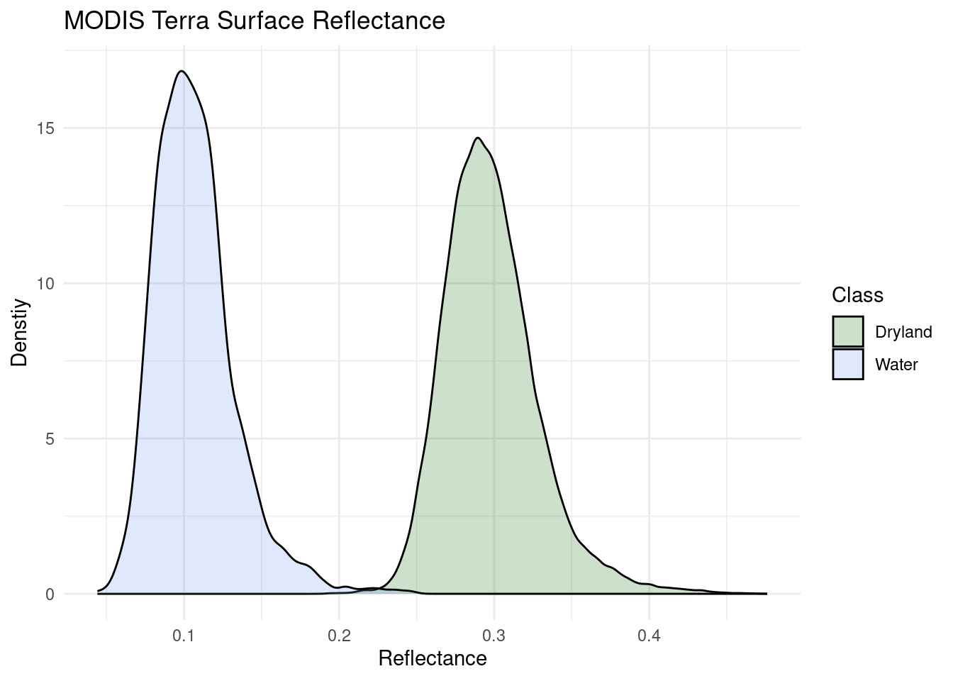

modis_specs(flood_wet)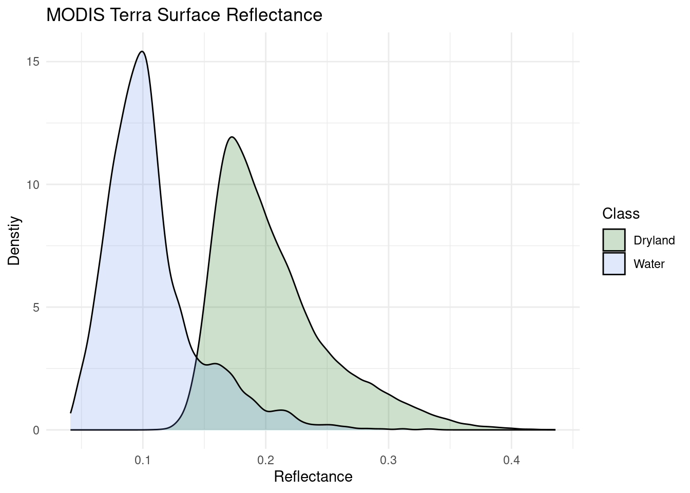

In our case, it appears that only the first map is bimodal, whereas the second is not. This can quite clearly be seen from the spectral reflectance images that show a substantial overlap in the second case. For the sake of this tutorial, we’ll ignore the bimodality issue.

Classifying an Image

We can now go ahead and run a classification to create a proper flood map. For this, we use the modis_classify() function, which will automatically determine a threshold to split the map into dryland and water. If the map fails the bimodality check, we can still enforce a classification using the option ignore.bimodality = T. However, this is not advised and may result in unreliable flood maps.

# Classify floodmaps, for now ignoring bimodality
flood_dry_class <- modis_classify(flood_dry, ignore.bimodality = T)
flood_wet_class <- modis_classify(flood_wet, ignore.bimodality = T)

# Visualize the classified maps
par(mfrow = c(1, 2))
plot(flood_dry_class, col = c("white", "cornflowerblue"), main = "Flood 2022-09-16")
plot(flood_wet_class, col = c("white", "cornflowerblue"), main = "Flood 2023-03-10")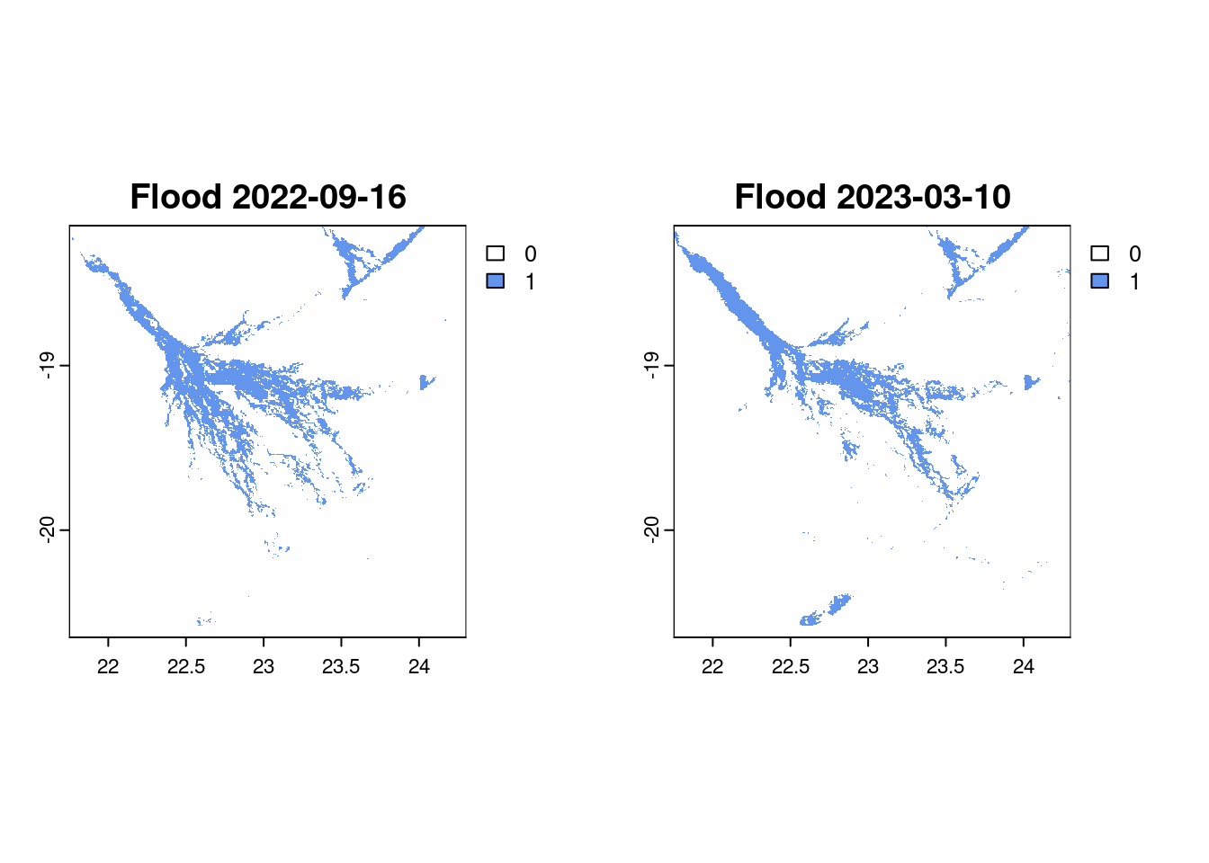

Figure 4: Classified flood maps.

Conclusion

With the floodmapr package were able to generate flood maps for a couple of dates with only few lines of code.

Session Information

## R version 4.1.2 (2021-11-01)
## Platform: x86_64-pc-linux-gnu (64-bit)
## Running under: Linux Mint 21.3
## 
## Matrix products: default
## BLAS:   /usr/lib/x86_64-linux-gnu/blas/libblas.so.3.10.0
## LAPACK: /usr/lib/x86_64-linux-gnu/lapack/liblapack.so.3.10.0
## 
## locale:
##  [1] LC_CTYPE=de_CH.UTF-8       LC_NUMERIC=C              
##  [3] LC_TIME=de_CH.UTF-8        LC_COLLATE=de_CH.UTF-8    
##  [5] LC_MONETARY=de_CH.UTF-8    LC_MESSAGES=de_CH.UTF-8   
##  [7] LC_PAPER=de_CH.UTF-8       LC_NAME=C                 
##  [9] LC_ADDRESS=C               LC_TELEPHONE=C            
## [11] LC_MEASUREMENT=de_CH.UTF-8 LC_IDENTIFICATION=C       
## 
## attached base packages:
## [1] stats     graphics  grDevices utils     datasets  methods   base     
## 
## other attached packages:
## [1] floodmapr_0.0.0.9000 raster_3.6-20        sp_1.6-1            
## 
## loaded via a namespace (and not attached):
##  [1] Rcpp_1.0.11      bslib_0.5.0      compiler_4.1.2   pillar_1.9.0    
##  [5] jquerylib_0.1.4  highr_0.10       tools_4.1.2      digest_0.6.31   
##  [9] timechange_0.2.0 lubridate_1.9.3  jsonlite_1.8.5   evaluate_0.21   
## [13] lifecycle_1.0.4  tibble_3.2.1     gtable_0.3.3     lattice_0.20-45 
## [17] pkgconfig_2.0.3  rlang_1.1.2      cli_3.6.1        rgdal_1.6-6     
## [21] curl_5.0.1       yaml_2.3.7       blogdown_1.17    xfun_0.39       
## [25] fastmap_1.1.1    terra_1.7-74     withr_2.5.2      httr_1.4.6      
## [29] dplyr_1.1.3      knitr_1.43       generics_0.1.3   sass_0.4.6      
## [33] vctrs_0.6.4      tidyselect_1.2.0 grid_4.1.2       glue_1.6.2      
## [37] R6_2.5.1         fansi_1.0.5      rmarkdown_2.22   bookdown_0.34   
## [41] farver_2.1.1     purrr_1.0.2      tidyr_1.3.0      ggplot2_3.4.4   
## [45] magrittr_2.0.3   scales_1.2.1     codetools_0.2-18 htmltools_0.5.5 
## [49] colorspace_2.1-0 labeling_0.4.2   utf8_1.2.4       munsell_0.5.0   
## [53] cachem_1.0.8