Introduction

Every observed movement trajectory can be viewed as a sequence of step-lengths and turning angles. The basic idea of Hidden Markov Movement Models (HMMMs) is to decompose this sequence into distinct behavioral modes by parametrizing step-length and turning-angle distributions that depend on the animal’s unobserved behavioral state. Stated differently, the idea is to find step-length and turning-angle distributions for a given number of states such that the likelihood of observing the collected data is maximized. Once the maximum likelihood estimates have been found, the “Viterbi-Algorithm” can be applied to retrieve the animal’s inferred movement state at every point in time. In movement ecology, HMMMs are very popular because they allow to connect observed movements to an unobserved underlying behavioral state.

In this blog post, we will simulate some movement data with known parameters and then fit an HMMM to see whether we can actually retrieve the correct simulation parameters using the moveHMM package.

Simulation Prerequisites

Let’s get started and set up our R-Session. First, we’ll load all packages that we need for this little project. To simulate a virtual landscape, we will use the brilliant NLMR package, which unfortunately is not available from CRAN. However, you can install it from github using:

# Install required r-packages
devtools::install_github("cran/RandomFields") # Dependency of NLMR, but not on CRAN
devtools::install_github("ropensci/NLMR")     # Not on CRAN

# Load required packages
library(tidyverse)   # For easier data handling
library(NLMR)        # To simulate landscapes
library(raster)      # To handle spatial data
library(moveHMM)     # To analyse the simulated data
library(ggpubr)      # To arrange multiple ggplot objects

Let’s generate a virtual landscape across which we can simulate some movement. Here, we’ll use a simple gaussian-field to represent a food-resource. It will determine the state-switching probabilities of our simulated animals, That is, depending on food-availability, our animals will be more or less likely to switch from one state to another (hence to change their movement mode).

# Simulate a resource (determines the likelihood of switching states)
food   <- raster(ncol = 500, nrow = 500, xmn = 0, xmx = 1000, ymn = 0, ymx = 1000)
food[] <- values(nlm_gaussianfield(ncol = 500, nrow = 500))
food   <- scale(food)

# Visualize it
ggplot(as.data.frame(food, xy = T), aes(x = x, y = y, fill = layer)) +
  geom_raster() +
  scale_fill_viridis_c(name = "Food Availability") +
  coord_equal() +
  theme_minimal() +
  theme(legend.position = "bottom") +
  guides(fill = guide_colourbar(title.position="top", title.hjust = 0.5))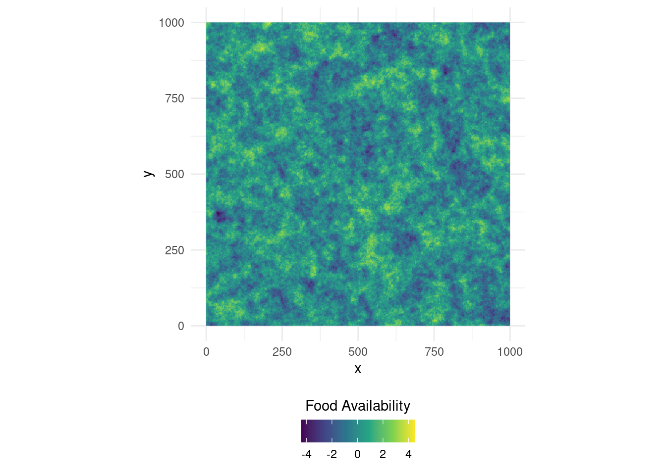

To now simulate movement across this landscape, we need three ingredients. (1) A function to sample step lengths, (2) a function to sample turning angles, and (3) a function to determine transition probabilities

Function to Sample Step Lengths

To sample step lengths we will simply use the gamma distribution. The gamma distribution has two parameters (shape and scale) and is often used in movement ecology because it matches observed movement patterns quite well. It’s mean and standard deviation are given by \[mean = shape * scale\] \[sd = shape^{0.5} * scale\]

Let’s take a look at some step lengths drawn from a gamma distribution for two hypothetical states (e.g. resting vs. moving).

# Simulate step lengths for two hypothetical states
states <- tibble(
    State = rep(c("State 1", "State 2"), each = 500)
  , Shape = ifelse (State == "State 1", 2.5, 3.0)
  , Scale = ifelse (State == "State 1", 0.5, 1.5)
  , StepLength = NA
)
for (i in 1:nrow(states)) {
  states$StepLength[i] <- rgamma(1, shape = states$Shape[i], scale = states$Scale[i])
}

# Visualize
ggplot(states, aes(x = StepLength)) +
  geom_histogram(col = "white", bins = 20, fill = "cornflowerblue") +
  theme_minimal() +
  xlab("Step Length") +
  facet_wrap(~ State)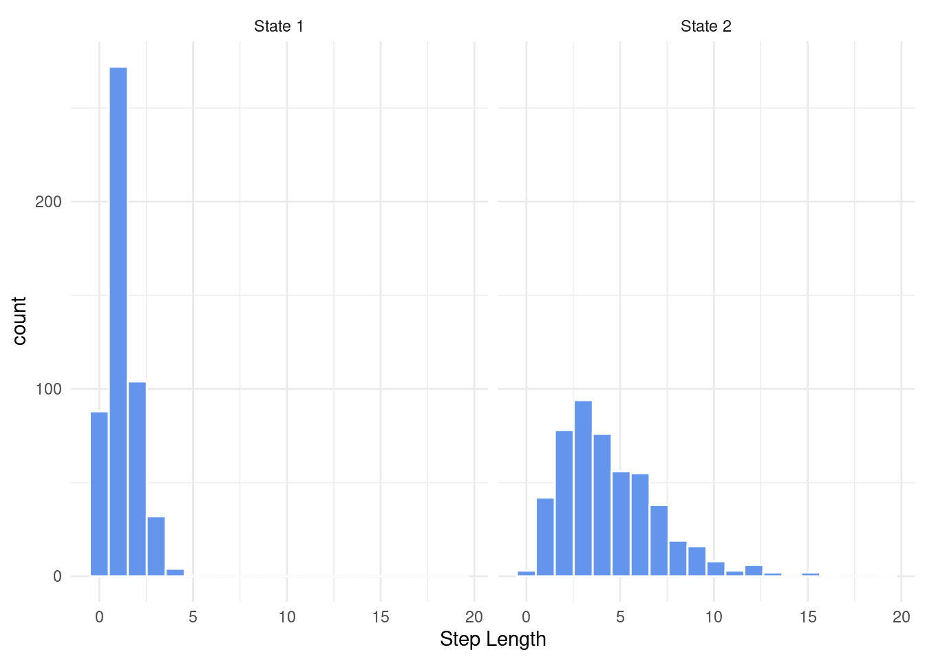

Function to Sample Turning Angles

Aside from sampling step lengths, we also need to be able to sample turning angles. The von Mises distribution is perfectly suited for this, as it is bound between \(-\pi\) and \(\pi\) and allows to render a tendency to move directional. It has a concentration parameter kappa and a location parameter mu. Because R neither provides a density function nor a random number generator for the von Mises distribution, we have to write those ourselves.

# Function to determine the probability density of a von Mises distribution
dvonmises <- function(x, kappa, mu, log = F) {
  d <- exp(kappa * cos(x - mu)) / (2 * pi * besselI(kappa, nu = 0))
  if (log == T) {
    d <- log(d)
  }
  return(d)
}

# Function to randomly sample values from a von Mises distribution
rvonmises <- function(n, kappa, mu, by = 0.01) {
  x <- seq(-pi, +pi, by = by)
  probs <- dvonmises(x, kappa = kappa, mu = mu)
  random <- sample(x, size = n, prob = probs, replace = T)
  return(random)
}

# Simulate turning angles for two hypothetical states
states <- tibble(
    State = rep(c("State 1", "State 2"), each = 500)
  , Kappa = ifelse (State == "State 1", 0.2, 0.5)
  , Mu    = 0
  , TurningAngle = NA
)
for (i in 1:nrow(states)) {
  states$TurningAngle[i] <- rvonmises(1, kappa = states$Kappa[i], mu = states$Mu[i])
}

# Visualize
ggplot(states, aes(x = TurningAngle)) +
  geom_histogram(col = "white", bins = 20, fill = "cornflowerblue") +
  theme_minimal() +
  xlab("Turning Angle") +
  facet_wrap(~ State)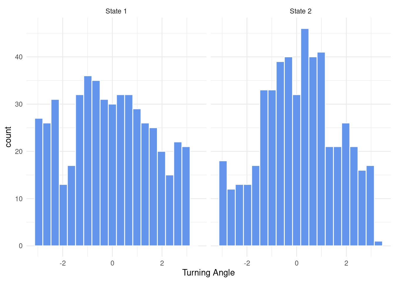

Function to Determine Transition-Probabilities

Finally, we need a function that governs the transition probabilities to switch from one state to another given a certain amount of food-availability. What we want is a function that takes a linear predictor and spits out a probability. A useful formula to turn a linear predictor (i.e. \(a + b * x\)) into a probability is the inverse of the logit. Hence, let’s write it down.

# Function to compute the transition probability, depending on food-availability
# and parameters a and b
transition <- function(food, a, b) {
  linear_predictor <- a + b * food
  1 / (1 + exp(-linear_predictor)) # Inverse logit
}

# Generate transition probability for different food-availability
tr <- tibble(
    Food = seq(-4, 4, by = 0.01)
  , TransitionProbability = transition(Food, a = 1, b = 2)
)

# Function to sample a state
sample_state <- function(state, food) {
  p <- transition(food, params$T_a[state], params$T_b[state])
  change <- rbinom(n = 1, size = 1, prob = p)
  if (state == 1 & change == 1) {
    state <- 2
  } else if (state == 2 & change == 1) {
    state <- 1
  }
  return(state)
}

# Visualize
ggplot(tr, aes(x = Food, y = TransitionProbability)) +
  geom_line(col = "cornflowerblue", lwd = 1.2) +
  ylab("Transition Probability") +
  theme_minimal()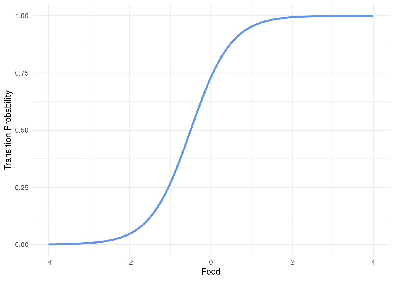

Simulation Parameters

We are now ready to put the different building blocks together and start our movement simulation. First, we define the different movement parameters that will be used in the simulation.

# Number of steps to simulate
n_steps <- 100

# Number of individuals to simulate
n_indivs <- 100

# Create tibble (a fancy dataframe) into which we will store the results
sims <- tibble(ID = 1:n_indivs)

# Movement parameters
params <- tibble(
    State     = c("Resting", "Moving")
  , GammaMean = c(5, 15)   # Mean of the gamma distribution
  , GammaSD   = c(5, 10)   # Standard deviation of the gamma distribution
  , MisesMean = c(0, 0)    # Mean (location) of the von Mises distribution
  , MisesCon  = c(0.5, 1)  # Concentration parameter of the von Mises distribution
  , T_a       = c(1, 2)    # Intercept of the linear predictor for transition probs.
  , T_b       = c(-1, 4)   # Slope of the linear predictor for transition probs.
)

Given this set of parameters, we can visualize the step lengths, turning angles and transition probabilities that we will expect. This is simply to ensure that everything works fine and that we’re not generating unreasonable data.

# Compute probability density functions for step lengths, turning angles, and
# transition probabilities for the given simulation parameters
example <- params %>%
  mutate(StepLengths = map2(GammaMean, GammaSD, function(x, y) {
    tibble(
        StepLength = seq(0, 60, length.out = 1000)
      , Density    =  dgamma(StepLength, shape = (x / y) ** 2, scale = y ** 2 / x)
    )
  })) %>%
  mutate(TurningAngles = map2(MisesCon, MisesMean, function(x, y) {
    tibble(
        TurningAngle = seq(-pi, +pi, length.out = 1000)
      , Density      = dvonmises(TurningAngle, kappa = x, mu = y)
    )
  })) %>%
  mutate(Transitions = map2(T_a, T_b, function(x, y) {
    tibble(
        Food    = seq(-4, +4, length.out = 1000)
      , Density = transition(Food, x, y)
    )
  }))

# Visualize
p1 <- example %>%
  unnest(StepLengths) %>%
  ggplot(aes(x = StepLength, y = Density)) +
    geom_line(col = "cornflowerblue", lwd = 1.2) +
    facet_wrap(~State) +
    theme_minimal() +
    xlab("Step Length")
p2 <- example %>%
  unnest(TurningAngles) %>%
  ggplot(aes(x = TurningAngle, y = Density)) +
    geom_line(col = "cornflowerblue", lwd = 1.2) +
    facet_wrap(~State) +
    theme_minimal() +
    xlab("Turning Angle")
p3 <- example %>%
  unnest(Transitions) %>%
  ggplot(aes(x = Food, y = Density)) +
    geom_line(col = "cornflowerblue", lwd = 1.2) +
    facet_wrap(~State) +
    theme_minimal() +
    ylab("Transition Probability")

# Put the plots together
ggarrange(p1, p2, p3, nrow = 3)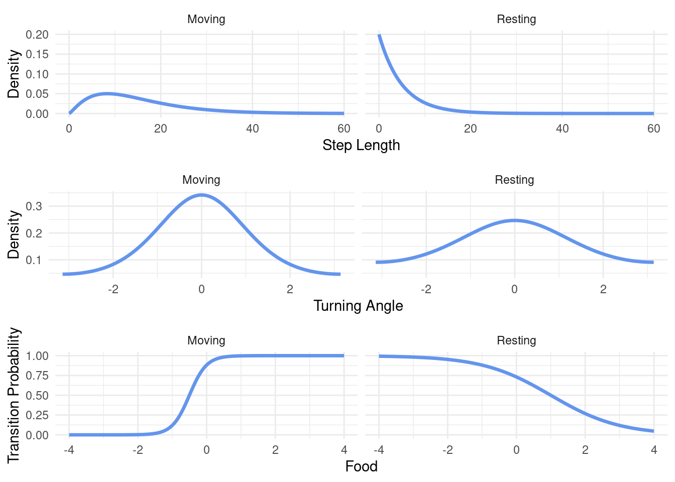

This looks good! When the animal is in the “Moving” state, the step lengths tend to be larger, turning angles tend to be narrower (closer to 0) and the transition probability reacts quite strongly to changes in food-availability. In contrast, when the animal is resting, step lengths tend to be short, turning angles less concentrated around 0 (still with a tendency to move forward though) and the transition probability reacts less strongly to changes in the food-availability.

With this we can finally run our movement simulation. The simulation works as follows:

An animal is released at the center of the map at \((x, y) = (500, 500)\) and is assumed to be oriented towards north
Food-availability at the animal’s current location is extracted and a new state is determined. The animal can either switch state or remain in the current state. Transition probabilities depend on the food availability.
A random step length and random turning angle are sampled from the distributions of the respective state.
The new position of the animal is calculated Steps 2 to 4 are then repeated until a total of 100 steps are simulated.

To run the simulation for all 100 individuals, we use the lapply() function, which is basically a “for-loop” that returns a list. For easier “bookkeeping” of the list, we can make use of tibbles. Tibbles are incredibly powerful versions of dataframes and make it fairly easy to keep track of our simulation outputs. They allow us to store the simulated data of different individuals into a single column titled “Simulations”. The rest of the code should be self-explanatory.

# Run simulations
sims$Simulations <- lapply(1:nrow(sims), function(x) {

  # Generate dataframe to keep track of coordinates and other data
  df <- data.frame(
      x     = rep(NA, n_steps) # x-coordinate
    , y     = rep(NA, n_steps) # y-coordinate
    , stepl = rep(NA, n_steps) # Step length
    , relta = rep(NA, n_steps) # Relative turning angle (heading / orientation)
    , absta = rep(NA, n_steps) # Absolute turning angle
    , state = rep(NA, n_steps) # Current state
    , food  = rep(NA, n_steps) # Food-availability
  )

  # Specify an initial orientation and state
  absta_init <- 0
  state_init <- 1

  # Initiate first rows of the dataframe (animal is released at the center)
  df$x[1] <- 500
  df$y[1] <- 500

  # Generate the movement trajectory based on random step lengths and turning
  # angles
  for (i in 1:(nrow(df) - 1)) {
    
    # Determine food availability
    f <- raster::extract(food, cbind(df$x[i], df$y[i]))
    
    # Determine the animal's new state
    s <- sample_state(state_init, f)
    
    # Sample step lengths from the state-specific gamma distribution
    df$stepl[i] <- rgamma(1
      , shape = (params$GammaMean[s] / params$GammaSD[s]) ** 2
      , scale = params$GammaSD[s] ** 2 / params$GammaMean[s]
    )
    
    # Sample (relative) turning angles from the state-specific von mises
    # distribution
    df$relta[i] <- rvonmises(1
      , mu    = params$MisesMean[s]
      , kappa = params$MisesCon[s]
    )
    
    # Compute the absolute turning angle
    df$absta[i] <- absta_init + df$relta[i]
    
    # Compute the new location of the animal
    df$x[i + 1] <- df$x[i] + sin(df$absta[i]) * df$stepl[i]
    df$y[i + 1] <- df$y[i] + cos(df$absta[i]) * df$stepl[i]
    
    # Store other relevant information
    df$food[i]  <- f
    df$state[i] <- s
    absta_init  <- df$absta[i]
    state_init  <- df$state[i]
  }

  # Return the simulation
  return(df)
})

The simulation shouldn’t take longer than a couple of seconds. Note that the final tibble is nested, i.e. all simulated data of single individual is contained within that specific individual’s row. Hence, we want to unnest the tibble to get a regular dataframe.

# Unnest the data
sims <- unnest(sims, Simulations)

# Take a look at the unnested data
head(sims)

## # A tibble: 6 × 8
##      ID     x     y stepl  relta absta state   food
##   <int> <dbl> <dbl> <dbl>  <dbl> <dbl> <dbl>  <dbl>
## 1     1  500   500   2.60  0.828 0.828     1  1.18 
## 2     1  502.  502. 19.6   0.148 0.977     2  0.739
## 3     1  518.  513. 20.8  -0.422 0.555     1 -0.606
## 4     1  529.  530. 28.9   2.80  3.35      2 -0.764
## 5     1  523.  502.  4.15 -1.09  2.26      2 -1.27 
## 6     1  526.  499. 12.8  -0.892 1.37      2 -2.12

You can see that unnesting preserves the simulation ID which is super-convenient because we can use it to distinguish different individuals. We can now visualize the simulated trajectories on a map. Remember that we released all individuals at the center, which is why it will by quite crowded there!

# Visualize it
ggplot() +
  geom_raster(data = as.data.frame(food, xy = T), aes(x = x, y = y, fill = layer)) +
  scale_fill_viridis_c(name = "Food Availability") +
  geom_point(data = sims, aes(x = x, y = y, group = as.factor(ID)), size = 0.5) +
  geom_path(data = sims, aes(x = x, y = y, group = as.factor(ID)), linewidth = 0.5) +
  coord_equal() +
  theme_minimal() +
  theme(legend.position = "bottom") +
  guides(fill = guide_colourbar(title.position="top", title.hjust = 0.5))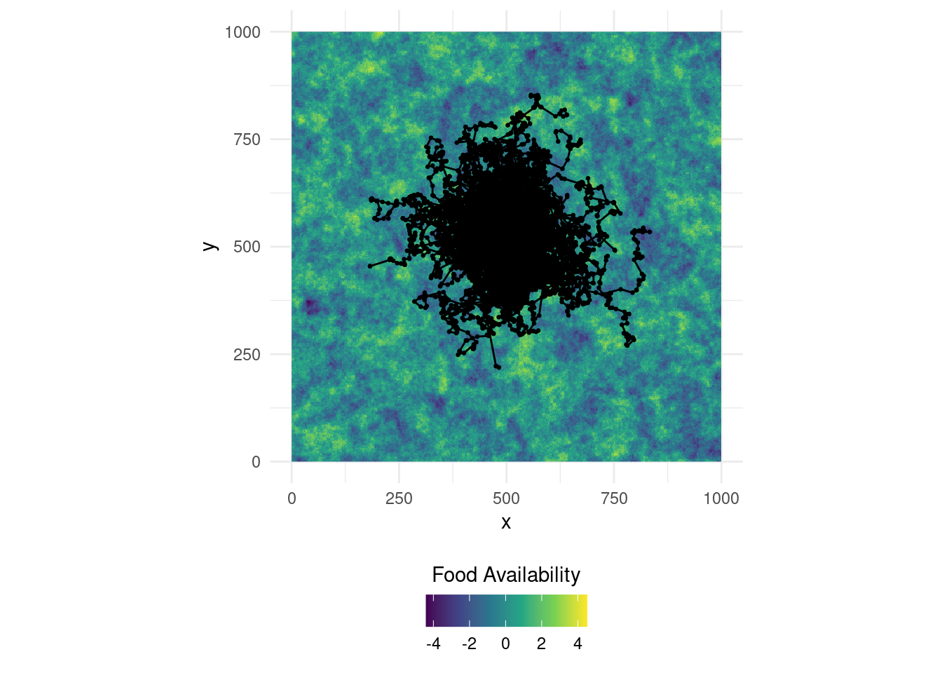

Fitting the Model

With the simulated data we can finally go ahead and fit a hidden markov movement model. If everything works correctly, we should be able to obtain exactly the input parameters that we used to simulate movement. First, however, we need to make sure the data is in the correct format. We can do this using the prepData() function.

# Prepare the data (ignore the warning)
df_prep <- prepData(as.data.frame(sims[, c("ID", "x", "y", "food")])
  , type       = "UTM"
  , coordNames = c("x", "y")
)

For the optimizer to work, we will need to provide initial values. If you want to learn more about how to chose initial values, I would recommend you to read the following vignette but the basic idea is to plot histograms of the observed values and then to set plausible initial values accordingly. Note that for the gamma distribution the package does not take the shape and scale parameters, but requires us to provide a mean and standard deviation instead (the formulas to compute mean and standard deviation from the shape and scale of a gamma distribution are given above).

# Histogram of step lengths and turning angles
p1 <- ggplot(df_prep, aes(x = step)) +
  geom_histogram(col = "white", fill = "cornflowerblue", bins = 20) +
  theme_minimal() +
  xlab("Step Length")
p2 <- ggplot(df_prep, aes(x = angle)) +
  geom_histogram(col = "white", fill = "cornflowerblue", bins = 20) +
  theme_minimal() +
  xlab("Turning Angle")
ggarrange(p1, p2, nrow = 1)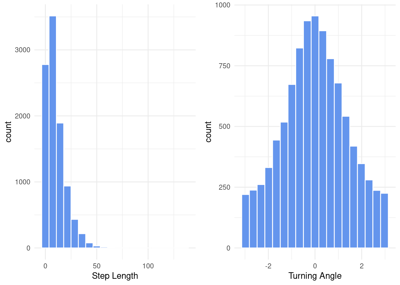

# Define initial values for step length distribution(s)
mu0 <- c(5, 10)    # Resting (5) and moving (10) parameters
sd0 <- c(5, 10)    # Resting (5) and moving (10) parameters
stepPar <- c(mu0, sd0)

# Define intial values for turning angle distribution(s)
anglemean0 <- c(0, 0)  # Resting (0) and moving (0) parameters
anglecon0 <- c(0.5, 1) # Resting (0) and moving (0) parameters
anglePar <- c(anglemean0, anglecon0)

We can now go ahead and fit the model to estimate the parameters of interest. Note that we provide a model formula indicating that we believe that the transition probabilities depend on food-availability. We also need to tell the model for how many states it should try to assign. In most applications people use two states only (e.g. resting and moving).

# Fit the model
mod <- fitHMM(
    data      = df_prep
  , nbStates  = 2
  , stepPar0  = stepPar
  , anglePar0 = anglePar
  , formula   = ~ food
)

Let’s put the true parameters and the estimates from the model side by side so that we can better verify that the model has done a good job.

# Compare step-length simulation parameters to estimates from moveHMM
list(mod$mle$stepPar, t(params[, c("State", "GammaMean", "GammaSD")]))

## [[1]]
##       state 1   state 2
## mean 5.080427 15.188335
## sd   5.102551  9.992704
## 
## [[2]]
##           [,1]      [,2]    
## State     "Resting" "Moving"
## GammaMean " 5"      "15"    
## GammaSD   " 5"      "10"

# Compare turning-angle simulation parameters to estimates from moveHMM
list(mod$mle$anglePar, t(params[, c("State", "MisesMean", "MisesCon")]))

## [[1]]
##                   state 1     state 2
## mean          0.003855044 0.001301972
## concentration 0.490353060 1.015617926
## 
## [[2]]
##           [,1]      [,2]    
## State     "Resting" "Moving"
## MisesMean "0"       "0"     
## MisesCon  "0.5"     "1.0"

# Compare transition-parameters to estimates from moveHMM
list(mod$mle$beta, t(params[, c("State", "T_a", "T_b")]))

## [[1]]
##               1 -> 2   2 -> 1
## intercept  0.9307734 2.033371
## food      -0.9901982 4.096431
## 
## [[2]]
##       [,1]      [,2]    
## State "Resting" "Moving"
## T_a   "1"       "2"     
## T_b   "-1"      " 4"

Impressive! The model almost perfectly approximated all of the true parameters. We might, however, also be interested in the derived states. For this, we can apply the Viterbi algorithm. We then compare the derived states to the true states.

# Compare states
states <- viterbi(mod)
cor(sims$state, states, use = "pairwise.complete.obs")

## [1] 0.7017736

# Confusion matrix
table(sims$state, states)

##    states
##        1    2
##   1 4036  826
##   2  651 4387

We can even plot the transition probabilities and will find that the plot looks almost identical to the one we produced in the beginning.

# Plot transition probs
plotStationary(mod, plotCI = T)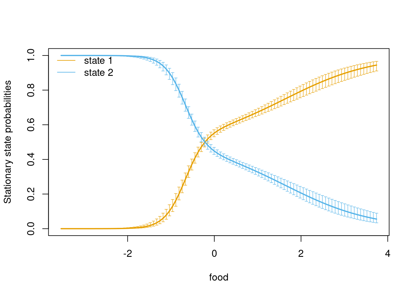

Conclusion

In this blog post we simulated 100 individuals moving across a virtual landscape. The individuals exhibited two distinct behavioral modes that determined their movement behavior. Using HMMMs implemented in the moveHMM package we successfully recovered all simulation parameters and could determine the behavioral modes with high accuracy.

Session Information

## R version 4.1.2 (2021-11-01)
## Platform: x86_64-pc-linux-gnu (64-bit)
## Running under: Linux Mint 21.3
## 
## Matrix products: default
## BLAS:   /usr/lib/x86_64-linux-gnu/blas/libblas.so.3.10.0
## LAPACK: /usr/lib/x86_64-linux-gnu/lapack/liblapack.so.3.10.0
## 
## locale:
##  [1] LC_CTYPE=de_CH.UTF-8       LC_NUMERIC=C              
##  [3] LC_TIME=de_CH.UTF-8        LC_COLLATE=de_CH.UTF-8    
##  [5] LC_MONETARY=de_CH.UTF-8    LC_MESSAGES=de_CH.UTF-8   
##  [7] LC_PAPER=de_CH.UTF-8       LC_NAME=C                 
##  [9] LC_ADDRESS=C               LC_TELEPHONE=C            
## [11] LC_MEASUREMENT=de_CH.UTF-8 LC_IDENTIFICATION=C       
## 
## attached base packages:
## [1] stats     graphics  grDevices utils     datasets  methods   base     
## 
## other attached packages:
##  [1] ggpubr_0.6.0    moveHMM_1.9     CircStats_0.2-6 boot_1.3-28    
##  [5] MASS_7.3-55     raster_3.6-20   sp_1.6-1        NLMR_1.1.1     
##  [9] lubridate_1.9.3 forcats_1.0.0   stringr_1.5.1   dplyr_1.1.3    
## [13] purrr_1.0.2     readr_2.1.4     tidyr_1.3.0     tibble_3.2.1   
## [17] ggplot2_3.4.4   tidyverse_2.0.0
## 
## loaded via a namespace (and not attached):
##  [1] httr_1.4.6            sass_0.4.6            jsonlite_1.8.5       
##  [4] viridisLite_0.4.2     carData_3.0-5         bslib_0.5.0          
##  [7] highr_0.10            yaml_2.3.7            numDeriv_2016.8-1.1  
## [10] pillar_1.9.0          backports_1.4.1       lattice_0.20-45      
## [13] glue_1.6.2            digest_0.6.31         ggsignif_0.6.4       
## [16] checkmate_2.2.0       colorspace_2.1-0      cowplot_1.1.1        
## [19] htmltools_0.5.5       plyr_1.8.8            pkgconfig_2.0.3      
## [22] broom_1.0.5           bookdown_0.34         scales_1.2.1         
## [25] terra_1.7-74          jpeg_0.1-10           tzdb_0.4.0           
## [28] timechange_0.2.0      ggmap_3.0.2           farver_2.1.1         
## [31] generics_0.1.3        car_3.1-2             cachem_1.0.8         
## [34] withr_2.5.2           cli_3.6.1             magrittr_2.0.3       
## [37] evaluate_0.21         fansi_1.0.5           rstatix_0.7.2        
## [40] RandomFieldsUtils_0.5 blogdown_1.17         tools_4.1.2          
## [43] hms_1.1.3             geosphere_1.5-18      RgoogleMaps_1.4.5.3  
## [46] lifecycle_1.0.4       munsell_0.5.0         compiler_4.1.2       
## [49] jquerylib_0.1.4       rlang_1.1.2           grid_4.1.2           
## [52] RandomFields_3.3.1    labeling_0.4.2        bitops_1.0-7         
## [55] rmarkdown_2.22        gtable_0.3.3          codetools_0.2-18     
## [58] abind_1.4-5           R6_2.5.1              knitr_1.43           
## [61] fastmap_1.1.1         utf8_1.2.4            stringi_1.8.1        
## [64] Rcpp_1.0.11           vctrs_0.6.4           png_0.1-8            
## [67] tidyselect_1.2.0      xfun_0.39

A Simulation-Based Introduction to Hidden-Markov Movement Models