Update 2023

This blog post was updated on December 18, 2023 to reflect the latest updates to the MegaDetector.

Introduction

Cameratraps (Figure 1) have become an increasingly popular tool to monitor and study animal populations. One of the main reason why cameratraps have become so omnipresent in ecology is because they are non-invasive and, once set up, can be left in the field for months, requiring only only little maintenance. This enables a largely automated data collection that grants exciting insights into wildlife. On the downside, cameratraps can produce thousands of images that may require a trained biologists to identify species. This can be very time-consuming and cumbersome, particularly if many of the images are empty and do not contain any animals (false positives). Consequently, there is a growing interest towards automating such tedious processes with the aid of artificial intelligence.

Figure 1: A Brownings wildlife camera that I’ve set up in my garden to learn about our nocturnal visitors from the nearby forest.

With the uprise of deep learning techniques, such repetitive tasks can be efficiently tackled using computer vision. For cameratrap images in particular, Microsoft has produced a neural network called the “MegaDetector”. The MegaDetector is a powerful neural network that has been exposed to millions of images containing humans, vehicles, and animals, and therefore is able to recognize these categories with great accurracy. Even though the detector only detects these three categories, it has proven to be incredibly reliable. In fact, I repeatedly found myself outperformed, especially in cases where an animal is lingering in the background or the dark. The MegaDetector can therefore serve as a powerful first filter to remove empty images, thereby significantly reducing the amount of images that need to be visually inspected by a human being, or to be further processed by a species identification AI. In this blog-post, I will to outline a simple workflow that allows you to apply the MegaDetector to your own set of images and to retrieve a list of identified objects in your images. Ultimately, I will show you how to import the so generated detections into R and how to visualize the detections.

Installation

Probably the most difficult part of using the MegaDetector is to set everything up. Hence, this blog-post will be primarily aimed towards helping you installing all required modules so you can get the MegaDetector to run on your machine. I will try to remain as simple as possible, but as thorough as needed. If you’re keen on learning more about the details of the MegaDetector, I suggest you take a look at either Microsoft’s Github Instructions or Dan Morris’ Tutorial. Microsoft and Dan are both providing great resources, but I’ll here focus on the one’s provided by Dan, as they appear more straight-forward to me.

# Create the "Megadetector" folder into which we'll download the files. The
# exact path will be different for you.
mkdir /home/david/Schreibtisch/Megadetector
cd /home/david/Schreibtisch/Megadetector

# Download required folders from GitHub
git clone https://github.com/ecologize/yolov5
git clone https://github.com/ecologize/CameraTraps
git clone https://github.com/Microsoft/ai4eutils

# Also download the Megadetector Models
wget https://github.com/microsoft/CameraTraps/releases/download/v5.0/md_v5a.0.0.pt
wget https://github.com/microsoft/CameraTraps/releases/download/v5.0/md_v5b.0.0.pt

# (Optional) Download my bash script for running the MegaDetector
wget https://raw.githubusercontent.com/DavidDHofmann/RunMegaDetector/main/RunMegaDetector.sh

# (Optional) Download sample images
git clone https://github.com/DavidDHofmann/SampleImages

# Specify a directory
directory <- "/home/david/Schreibtisch/Megadetector"

# Check if the directory already exists
if (!dir.exists(directory)) {
  dir.create(directory)
}

# Adjust timeout
options(timeout = 600)

# Download folders
files <- c("yolov5", "cameratraps", "ai4eutils", "SampleImages")
exist <- file.exists(file.path(directory, files))
files <- files[!exist]
for (i in files) {
  if (i == "yolov5") {
      url = "https://github.com/ecologize/yolov5/archive/refs/heads/master.zip"
    } else if (i == "cameratraps") {
      url = "https://github.com/ecologize/CameraTraps/archive/refs/heads/master.zip"
    } else if (i == "ai4eutils") {
      url = "https://github.com/Microsoft/ai4eutils/archive/refs/heads/master.zip"
    } else {
      url = "https://github.com/DavidDHofmann/SampleImages/archive/refs/heads/main.zip"
  }
  download.file(
      url      = url
    , destfile = file.path(directory, paste0(i, ".zip"))
  )

  # Unzip the .zip files
  zipname <- basename(unzip(file.path(directory, paste0(i, ".zip")), list = T)$Name[1])
  unzip(file.path(directory, paste0(i, ".zip")), exdir = directory)
  file.rename(from = file.path(directory, zipname), to = file.path(directory, i))
  file.remove(file.path(directory, paste0(i, ".zip")))

}

# Download models
download.file(
    url      = "https://github.com/microsoft/CameraTraps/releases/download/v5.0/md_v5a.0.0.pt"
  , destfile = file.path(directory, "md_v5a.0.0.pt")
)
download.file(
    url      = "https://github.com/microsoft/CameraTraps/releases/download/v5.0/md_v5b.0.0.pt"
  , destfile = file.path(directory, "md_v5b.0.0.pt")
)

# We also need to install the bashscript to initiate the megadetector
download.file(
    url = "https://raw.githubusercontent.com/DavidDHofmann/RunMegaDetector/main/RunMegaDetector.sh"
  , destfile = file.path(directory, "RunMegaDetector.sh")
)

CameraTrapping
└───ai4eutils
    └───...
└───cameratraps
    └───...
└───yolov5
    └───...
└───SampleImages
    │ L002_R01_20210307212248.JPG
    │ L002_R01_20210308022921.JPG
    │ ...
    └───Detections
│   md_v5a.0.0.pt
│   md_v5b.0.0.pt
│   RunMegaDetector.sh

# In brackets, mamba always tells you in which environment you are working
(base) david@minty:~$

# On Linux / Windows
'mamba env create --file cameratraps/envs/environment-detector.yml'

# On Mac, pick one of the following
'mamba env create --file cameratraps/envs/environment-detector-m1.yml'
'mamba env create --file cameratraps/envs/environment-detector-mac.yml'
'mamba env create --file cameratraps/envs/environment-detector-mac-nomkl.yml'

Running the MegaDetector

mamba activate cameratraps-detector

# In brackets, mamba always tells you in which environment you are working
(cameratraps-detector) david@minty:~$

# Make folders available to python
export PYTHONPATH="$PYTHONPATH:cameratraps:ai4eutils:yolov5"

Classifying Images

There are several different ways in which we can run the MegaDetector:

• Approach I: We could use the run_tf_detector.py script (stored under cameratraps/detection), which automatically runs the detection algorithm and creates one or multiple images with bounding boxes drawn around all detections. This approach is useful if you want to test the MegaDetector on a couple of example images. However, it is not very useful for large number of files because the detection information is not stored in a structured manner and therefore can’t be used for further analysis.

• Approach II: We could also use the run_tf_detector_batch.py script (stored under cameratraps/detection), which runs the detection algorithm on a folder and returns a “list of lists” containing all detections found within the images of that folder. Conveniently, each detection has an associated uncertainty, showing us how “confident” the detector is for that specific detection. While this approach does not directly produce images with neat bounding boxes, it actually produces a file that can be further processed. It is therefore much more useful for scientific purposes. Bounding boxes can later be created, as I will show below. In addition, this script periodically saves the MegaDetector’s output, such that not all progress is lost if your classification session crashes.

Approach I

In this first approach, we use the run_tf_detector.py script and run it from our computer terminal. The script can either be applied to a single image or to an entire directory. In the latter case, the script will go through each image in the provided directory. Let’s first take a look at the anatomy of the commands that we’ll be using. The commands to invoke the python script are the following (you’ll need to fill in filename and directoryname yourself):

# If you want to run the detection on a single image
python cameratraps/detection/run_detector.py md_v5a.0.0.pt --image_file filename --output_dir directoryname

# If you want to run the detection on an entire directory
python cameratraps/detection/run_detector.py md_v5a.0.0.pt --image_dir directoryname --output_dir directoryname

Let me briefly explain what each element of these commands are doing:

• python cameratraps/detection/run_tf_detector.py tells our computer to run the run_tf_detector.py script using python.

• md_v5a.0.0.pt is our model file (i.e. the pre-trained neural network). You could also use the second model instead md_v5a.0.0.pt.

• --image_file filename allows us to specify the image on which we want to detect animals

• --image_dir directoryname allows us to specify the directory containing all images on which we want to detect animals

• --output_dir directoryname allows us to specify the directory into which the newly created images should be stored

Of course there are many other options that you may want to play with. To get the full list of available options, simply type:

# Show available options
python cameratraps/detection/run_tf_detector.py -h

Anyways, let’s run the detector on some real images. In case you have downloaded my example images, the commands from above translate into:

# Run MegaDetector on a single image
python cameratraps/detection/run_detector.py md_v5a.0.0.pt --image_file SampleImages/L002_R01_20210314013742.JPG --output_dir SampleImages/Detections

# Run MegaDetector on an entire directory
python cameratraps/detection/run_detector.py md_v5a.0.0.pt --image_dir SampleImages --output_dir SampleImages/Detections

If everything is setup correctly, the MegaDetector will get to work and run the detections for you. Once the algorithm terminates, you can go to the SampleImages/Detections folder where you should find the final images with bounding boxes around each detected animal/human/vehicle. The images should look something like shown in Figure 3b.

Figure 2: a) Input image and b) output image produced by the run_tf_detector.py script.

Nice! We just ran our first detection. Now let’s see how we can generate a list of detections instead.

Approach II

In this approach, we use the run_tf_batch_detector.py script. While this script does not generate neat looking pictures with bounding boxes, it creates a .json file that contains all the detections in a structured format. This allows us to import the file into R for further analysis. Again, let’s first look at the anatomy of the invoked command. To invoke the batch-detector script, we can use the following code (you’ll need to fill in filename/directory and outfilename.json by yourself):

# To run the MegaDetector batch file
python cameratraps/detection/run_detector_batch.py md_v5a.0.0.pt filename/directory outfilename.json

Again, we want to know what each piece of the code is doing.

• python cameratraps/detection/run_tf_detector_batch.py tells our computer to run the run_tf_detector_batch.py script using python.

• md_v5a.0.0.pt is our model file (i.e. the pre-trained neural network). You could also use the second model instead md_v5a.0.0.pt.

• SampleImages is the directory (or file) on which you want to run the megadetector.

• SampleImages/Detections.json is the output file into which the detections are stored.

For our sample images, this code snippet translates into:

# Run the MegaDetector and create a .json file
python cameratraps/detection/run_detector_batch.py md_v5a.0.0.pt SampleImages SampleImages/Detections.json

Again, the MegaDetector should get to work and start detecting animals. Depending on your computer and the number of images, this will take a while to complete. Luckily the MegaDetector gives you detailed information about its progress while its running.

The run_detector_batch.py offers many other options that you may want to play with. To get the full list of available options, simply type:

# Show available options
python cameratraps/detection/run_tf_detector_batch.py -h

Processing the MegaDetector Output

In case you run the run_tf_detector_batch.py, you’ll end up with a .json file containing all detections. You can of course open the file in a text-editor and try to go through the detections by hand. However, I strongly recommend to further process the file. Here, we will use R to import and clean the file and to visualize some of the detections. To load the file, we can use the fromJSON() function from the rjson package.

# Load required packages
library(rjson)      # To read a json file
library(tidyverse)  # For data wrangling
library(exifr)      # To read image meta-data
library(magick)     # To plot images
library(lubridate)  # To handle timestamps

# Load json file produced by the MegaDetector
anot <- fromJSON(file = "SampleImages/Detections.json")

Once the .json-file has been loaded, let’s take a look at its’ structure.

# Look at the structure of the json file
str(anot, 2)

## List of 3
##  $ images              :List of 10
##   ..$ :List of 2
##   ..$ :List of 2
##   ..$ :List of 2
##   ..$ :List of 2
##   ..$ :List of 2
##   ..$ :List of 2
##   ..$ :List of 2
##   ..$ :List of 2
##   ..$ :List of 2
##   ..$ :List of 2
##  $ detection_categories:List of 3
##   ..$ 1: chr "animal"
##   ..$ 2: chr "person"
##   ..$ 3: chr "vehicle"
##  $ info                :List of 4
##   ..$ detection_completion_time: chr "2024-03-23 16:26:40"
##   ..$ format_version           : chr "1.3"
##   ..$ detector                 : chr "md_v5a.0.0.pt"
##   ..$ detector_metadata        :List of 3

The file is basically a list of lists containing lots of information on the original input images, detected categories, and on the algorithm itself. We can consolidate all of this information into a single tibble/dataframe that is easier to read:

# Extract detected categories and put them into a tibble/dataframe
cats              <- enframe(anot$detection_categories)
names(cats)       <- c("CategoryID", "CategoryName")
cats$CategoryName <- unlist(cats$CategoryName)

# Get information into nice format
info <- tibble(
      images     = map_chr(anot$images, "file")
    , detections = lapply(anot$images, function(x){
      tibble(
          category   = map_chr(x$detections, "category")
        , confidence = map_dbl(x$detections, "conf")
        , bbox       = map(x$detections, "bbox")
      )
    })
  ) %>%
  unnest(detections) %>%
  mutate(bbox = map(bbox, function(x){paste0(x, collapse = ", ")})) %>%
  separate(bbox
    , sep     = ","
    , into    = c("x_left", "y_top", "x_width", "y_height")
    , convert = T
  )

# Join categories to the info table
info <- left_join(info, cats, by = c("category" = "CategoryID"))

# Look at the generated dataframe
head(info)

## # A tibble: 6 × 8
##   images        category confidence x_left   y_top x_width y_height CategoryName
##   <chr>         <chr>         <dbl>  <dbl>   <dbl>   <dbl>    <dbl> <chr>       
## 1 SampleImages… 3           0.00542  0     4.63e-3   0.156    0.457 vehicle     
## 2 SampleImages… 1           0.0245   0.886 7.61e-1   0.114    0.192 animal      
## 3 SampleImages… 2           0.962    0.361 9.26e-4   0.156    0.456 person      
## 4 SampleImages… 1           0.967    0.350 3.25e-1   0.279    0.294 animal      
## 5 SampleImages… 1           0.948    0.552 3.80e-1   0.308    0.403 animal      
## 6 SampleImages… 1           0.953    0.688 5.14e-1   0.294    0.440 animal

Awesome! Take a look at the output from the cleaned dataframe. It contains a row for each detection, so that if one image contains more than one detection, there will be multiple rows for the same image. By looking at the columns, we see that the file contains information on the detected categories (cateogry & CategoryName) and on the bounding boxes surrounding each of the detections. The bounding boxes are defined by an x and y coordinate (x_left & y_top) and a width and a height (x_width & y_height). Note that the respective numbers are given on a scale from 0 to 1, so that we’ll need to adjust the values depending on the image resolution. It is also important to note that in computer vision the y axis starts at the top and not from the bottom. Besides information on the detected category and the associated bounding box, we also see that for each detection the detector returned a measure of confidence (confidence). This is really useful because it allows us to subset to detections that exceed a desired threshold!

Now that we compiled all information into a nice table, we can conduct a wide range of exploratory analyses. For instance, we may want to identify all images on which the detector identified an animal with a relatively high confidence. We can easily subset to those images as follows:

# Identify images that contain animals
info %>%
  subset(CategoryName == "animal" & confidence > 0.9)

## # A tibble: 5 × 8
##   images          category confidence x_left y_top x_width y_height CategoryName
##   <chr>           <chr>         <dbl>  <dbl> <dbl>   <dbl>    <dbl> <chr>       
## 1 SampleImages/L… 1             0.967  0.350 0.325   0.279    0.294 animal      
## 2 SampleImages/L… 1             0.948  0.552 0.380   0.308    0.403 animal      
## 3 SampleImages/L… 1             0.953  0.688 0.514   0.294    0.440 animal      
## 4 SampleImages/L… 1             0.905  0     0.423   0.243    0.316 animal      
## 5 SampleImages/L… 1             0.945  0.438 0.382   0.194    0.192 animal

By default, the MegaDetector also returns detections for which he is very uncertain, which you can see by plotting a histogram of the “Confidence” values.

# Histogram of MegaDetectors confidence
hist(info$confidence
  , breaks = 10
  , main   = "Histogram of Confidence"
  , xlab   = "Confidence"
  , ylab   = "Frequency"
  , col    = "cornflowerblue"
  , border = NA
)

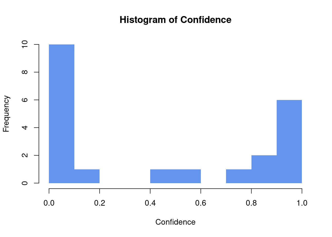
For now, we only want to consider detections with relatively high confidence. So let’s subset the data accordingly.

# Subset to detections with high confidence
info <- info %>%
  subset(confidence > 0.9)

You may also be interested during which time of the day you detected most animals. For this, we have to extract the timestamp of each cameratrap image. We can use the function read_exif() from the exifr package to extract such information from the image metadata. In fact, the function returns and entire dataframe of really useful information on each image that we may want to store for later.

# Load image metadata
meta <- read_exif(info$images)

# This contains a ton of information!
names(meta)

##  [1] "SourceFile"                 "ExifToolVersion"           
##  [3] "FileName"                   "Directory"                 
##  [5] "FileSize"                   "FileModifyDate"            
##  [7] "FileAccessDate"             "FileInodeChangeDate"       
##  [9] "FilePermissions"            "FileType"                  
## [11] "FileTypeExtension"          "MIMEType"                  
## [13] "ExifByteOrder"              "ImageDescription"          
## [15] "Make"                       "Model"                     
## [17] "Orientation"                "XResolution"               
## [19] "YResolution"                "ResolutionUnit"            
## [21] "Software"                   "ModifyDate"                
## [23] "YCbCrPositioning"           "Copyright"                 
## [25] "ExposureTime"               "FNumber"                   
## [27] "ExposureProgram"            "ISO"                       
## [29] "ExifVersion"                "DateTimeOriginal"          
## [31] "CreateDate"                 "ComponentsConfiguration"   
## [33] "CompressedBitsPerPixel"     "ShutterSpeedValue"         
## [35] "ApertureValue"              "ExposureCompensation"      
## [37] "MaxApertureValue"           "MeteringMode"              
## [39] "LightSource"                "Flash"                     
## [41] "FocalLength"                "Warning"                   
## [43] "UserComment"                "FlashpixVersion"           
## [45] "ColorSpace"                 "ExifImageWidth"            
## [47] "ExifImageHeight"            "InteropIndex"              
## [49] "InteropVersion"             "FileSource"                
## [51] "SceneType"                  "ExposureMode"              
## [53] "WhiteBalance"               "DigitalZoomRatio"          
## [55] "FocalLengthIn35mmFormat"    "SceneCaptureType"          
## [57] "Sharpness"                  "Compression"               
## [59] "ThumbnailOffset"            "ThumbnailLength"           
## [61] "MPFVersion"                 "NumberOfImages"            
## [63] "MPImageFlags"               "MPImageFormat"             
## [65] "MPImageType"                "MPImageLength"             
## [67] "MPImageStart"               "DependentImage1EntryNumber"
## [69] "DependentImage2EntryNumber" "ImageWidth"                
## [71] "ImageHeight"                "EncodingProcess"           
## [73] "BitsPerSample"              "ColorComponents"           
## [75] "YCbCrSubSampling"           "Aperture"                  
## [77] "ImageSize"                  "Megapixels"                
## [79] "ShutterSpeed"               "ThumbnailImage"            
## [81] "PreviewImage"               "FocalLength35efl"          
## [83] "LightValue"

# Extract timestamp and add it to our "info" table
info$Timestamp      <- as.POSIXct(meta$CreateDate, format = "%Y:%m:%d %H:%M:%S")
info$TimestampRound <- round(info$Timestamp, "hour")

# Identify number of detections depending on the time of the day
info %>%
  subset(CategoryName == "animal") %>%
  mutate(TimeOfDay = ifelse(hour(TimestampRound) %in% 6:22, "Day", "Night")) %>%
  count(TimeOfDay)

## # A tibble: 1 × 2
##   TimeOfDay     n
##   <chr>     <int>
## 1 Night         5

But back to the question of when we detected most animals. Here, it seems that only one of the eight detected animals appeared during the day. This is not really surprising, as I have rarely seen other animals than our cats during the day. Despite the useful information shown in the generated dataframe, you will often also want to visualize the detections. For this, we’ll need to load the respective image into R, draw a bounding box around the detected object and plot everything. We can write a function that allows us to automate these tasks:

# Function to plot the i-th image with bounding box around the detection
showDetection <- function(i = NULL){

  # Load ith image
  img  <- image_read(info$images[i])
  dims <- image_info(img)

  # Plot
  img <- image_draw(img)

  # Add bounding box around the detection (color depending on detected category)
  rect(
      xleft   = info$x_left[i] * dims$width
    , xright  = (info$x_left[i] + info$x_width[i]) * dims$width
    , ytop    = info$y_top[i] * dims$height
    , ybottom = (info$y_top[i] + info$y_height[i]) * dims$height
    , border  = c("red", "yellow", "green")[as.numeric(info$category[i])]
    , lwd     = 10
  )

  # Add a text label indicating the detected class (note that we ensure that the
  # label does not leave the image border on the y-axis).
  text(
      x      = info$x_left[i] * dims$width
    , y      = max(info$y_top[i], 0.05) * dims$height
    , labels = paste(info$CategoryName[i], info$confidence[i])
    , cex    = 5
    , col    = c("red", "yellow", "green")[as.numeric(info$category[i])]
    , adj    = c(0, 0)
  )

  # Add text indicating the image name
  text(
      0.5 * dims$width
    , 0.95 * dims$height
    , basename(info$images[i])
    , cex = 5
    , col = "white"
    , pos = 3
  )
  dev.off()
  plot(img)

}

# Let's try it on some example images
par(mfrow = c(3, 2), mar = c(0, 0, 0, 0))
plots <- lapply(1:6, function(i){showDetection(i)})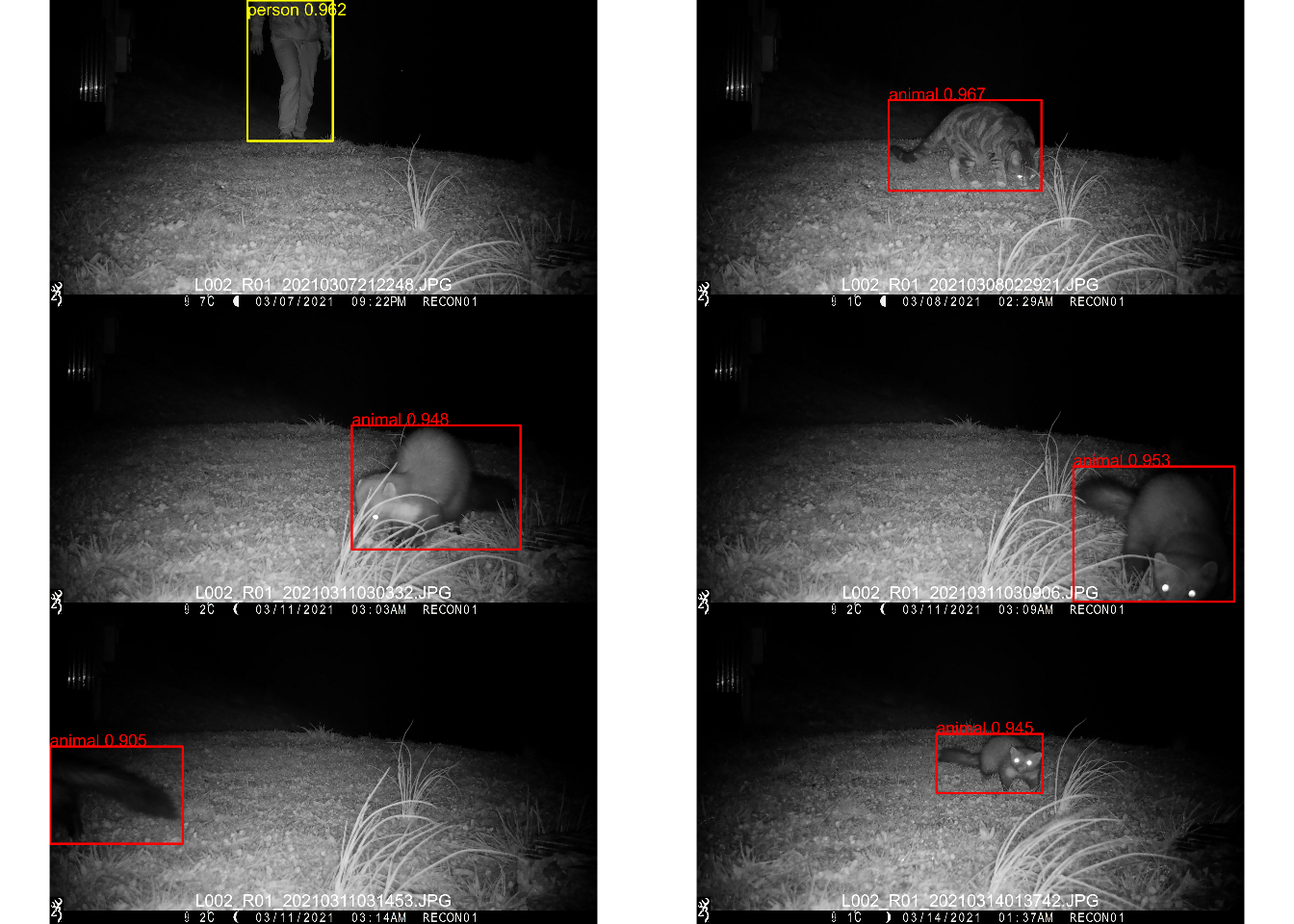

Figure 3: Some example detections on cameratrap images. Differently colored bounding boxes represent the different categories. The MegaDetector is able to distinguish animals, humans (person), and vehicles. As you can see on the image on the lower right, the detector even detects animals that are not fully within the picture!

Cool. It seems like the MegaDetector did a really nice job on our example images! Obviously the MegaDetector is not perfect and there will always be some misclassifications. Nevertheless, I am often very impressed by the MegaDetector’s ability to identify animals, even on low-light black and white images. It has happened to me multiple times that I skimmed through images and didn’t realize that an animal was lurking somewhere in the background, yet the MegaDetector picked it up perfectly! Nevertheless, if you’re using the MegaDetector for scientific purposes, definitely validate its output against some ground-truthed data ;)

Summary

Let’s summarize what we have learned in this blog post. We have explored how we can use the MegaDetector to easily identify animals on cameratrap images. We have also learned how we can import the .json output file into R to produce neat-looking images with bounding boxes around each detected animal. Overall, the MegaDetector is a very powerful and fun tool that allows us to automatically detect animals on cameratrap images.

Session Information

## R version 4.1.2 (2021-11-01)
## Platform: x86_64-pc-linux-gnu (64-bit)
## Running under: Linux Mint 21.3
## 
## Matrix products: default
## BLAS:   /usr/lib/x86_64-linux-gnu/blas/libblas.so.3.10.0
## LAPACK: /usr/lib/x86_64-linux-gnu/lapack/liblapack.so.3.10.0
## 
## locale:
##  [1] LC_CTYPE=de_CH.UTF-8       LC_NUMERIC=C              
##  [3] LC_TIME=de_CH.UTF-8        LC_COLLATE=de_CH.UTF-8    
##  [5] LC_MONETARY=de_CH.UTF-8    LC_MESSAGES=de_CH.UTF-8   
##  [7] LC_PAPER=de_CH.UTF-8       LC_NAME=C                 
##  [9] LC_ADDRESS=C               LC_TELEPHONE=C            
## [11] LC_MEASUREMENT=de_CH.UTF-8 LC_IDENTIFICATION=C       
## 
## attached base packages:
## [1] stats     graphics  grDevices utils     datasets  methods   base     
## 
## other attached packages:
##  [1] magick_2.7.4    exifr_0.3.2     lubridate_1.9.3 forcats_1.0.0  
##  [5] stringr_1.5.1   dplyr_1.1.3     purrr_1.0.2     readr_2.1.4    
##  [9] tidyr_1.3.0     tibble_3.2.1    ggplot2_3.4.4   tidyverse_2.0.0
## [13] rjson_0.2.21   
## 
## loaded via a namespace (and not attached):
##  [1] Rcpp_1.0.11      plyr_1.8.8       bslib_0.6.2      compiler_4.1.2  
##  [5] pillar_1.9.0     jquerylib_0.1.4  highr_0.10       tools_4.1.2     
##  [9] digest_0.6.35    timechange_0.2.0 jsonlite_1.8.8   evaluate_0.23   
## [13] lifecycle_1.0.4  gtable_0.3.3     pkgconfig_2.0.3  rlang_1.1.3     
## [17] cli_3.6.2        yaml_2.3.8       blogdown_1.17    xfun_0.42       
## [21] fastmap_1.1.1    withr_2.5.2      knitr_1.45       rappdirs_0.3.3  
## [25] hms_1.1.3        generics_0.1.3   sass_0.4.9       vctrs_0.6.4     
## [29] grid_4.1.2       tidyselect_1.2.0 glue_1.7.0       R6_2.5.1        
## [33] fansi_1.0.5      rmarkdown_2.26   bookdown_0.34    tzdb_0.4.0      
## [37] magrittr_2.0.3   scales_1.2.1     htmltools_0.5.7  colorspace_2.1-0
## [41] utf8_1.2.4       stringi_1.8.1    munsell_0.5.0    cachem_1.0.8