Introduction
When you visualize spatial data on a map, it is often useful to plot a satellite image in the background. Unfortunately, satellite data is incredibly expensive to produce, and so not every provider of corresponding data is willing to provide free access to it. Google, for instance, pays a lot of money to get access to satellite data of third parties, which it can then display on Google Maps or Google Earth. Consequently, you can only access its data using an API for which you potentially need to pay. Luckily, there are still other providers that grant access to satellite imagery for free. Hence, in today’s blog post, I would like to show you can access and download satellite imagery that is free of charge within R. Once downloaded, we will also learn how to plot the downloaded imagery using either base plot, ggplot, or the magnificent tmap package.
Downloading Satellite Imagery
Let’s assume that we want to visualize the study area of a research project that is located in the Swiss Alps on a satellite map. The area is given by the following rectangle:
# Load required packages for this blog post
library(raster)          # For handling spatial data
library(tmaptools)       # To download satellite imagery
library(GISTools)        # To add north arrow to a base plot
library(ggplot2)         # To plot using the ggplot engine
library(sf)              # To plot spatial objects with ggplot
library(ggspatial)       # To add north arrow and scale bars to a ggplot
library(tmap)            # To plot using tmap

# Rectangular polygon that delineates our study area
study_area <- as(extent(c(2762710, 2762905, 1184919, 1185332)), "SpatialPolygons")
crs(study_area) <- CRS("+init=epsg:2056")
We could now download satellite data for this region. However, I usually prefer to download data on a slightly larger extent so that some of the surroundings of the study area can also be included in the plot. Hence, let’s define an area of interest (aoi) for which we want to download satellite data.
# Define an area of interest (aoi)
aoi <- as(extent(c(2762179, 2763727, 1184568, 1185640)), "SpatialPolygons")
crs(aoi) <- CRS("+init=epsg:2056")

# Let's plot the study area and the area of interest together
plot(aoi, border = "blue", lty = 2)
plot(study_area, add = T, lty = 2, border = "red", col = adjustcolor("red", alpha.f = 0.2))
axis(1)
axis(2)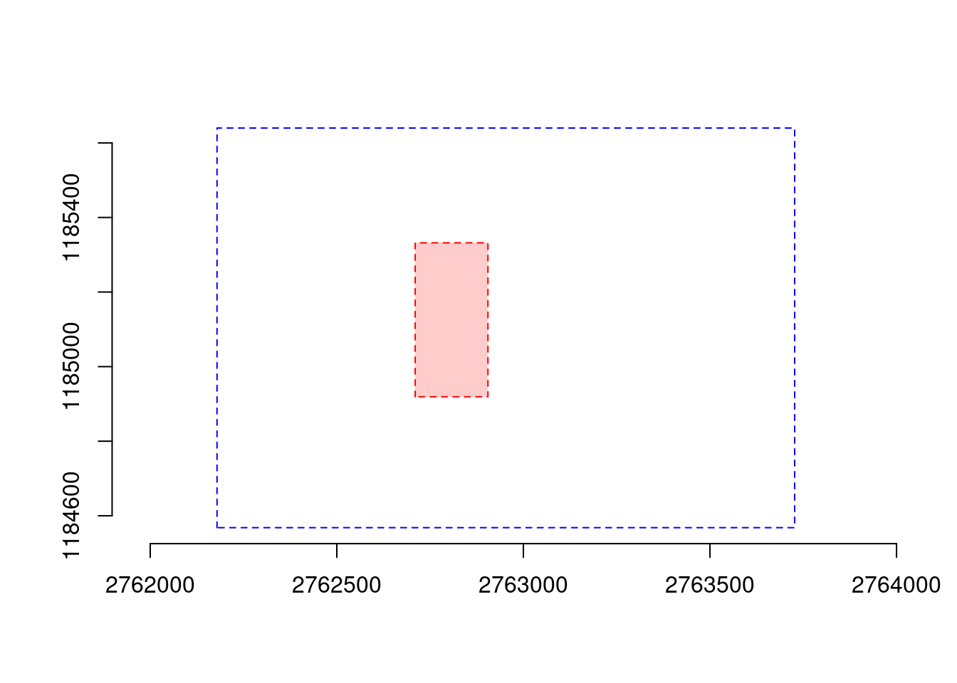
Neat! Now it’s time to download satellite data for the aoi. The package that
we’re going to use for this is called tmaptools (which in the background uses
the package OpenStreetMap). Instead of relying on satellite data provided
through Google, this package allows us to access satellite imagery from Bing
using the function read_osm() (in fact, you could access data for many other
providers too). The cool thing is that Bing enables us to download satellite
imagery at really high resolution. In fact, we can control the resolution of the
downloaded data by adjusting the zoom arguement. Let’s give it a try and
download some satellite data for our aoi.
# Download satellite data for the aoi (control resolution of the data using the
# "zoom" argument. The higher the number, the better the resolution but the
# longer the download will take)
sat <- read_osm(aoi, type = "bing", zoom = 17)

# Check what we downloaded
class(sat)
## [1] "stars"The downloaded object is of the class “stars”. I don’t really like this format,
so we’ll convert it to a regular raster-stack from the raster package. We will
also reproject the stack to the local LV-95 projection.
# Convert the downloaded satellite data to a rasterstack
sat <- as(sat, "Raster")

# Reproject the data to the correct CRS using the "nearest neighbor" (ngb)
# method
sat <- projectRaster(sat, crs = CRS("+init=epsg:2056"), method = "ngb")
The resulting raster-stack contains three raster layers, together forming an RGB image (band 1 = red, band 2 = green, band 3 = blue). Let’s take a look at each of the bands and plot them.
# Visualize the three layers
plot(sat, col = gray(0:100/100))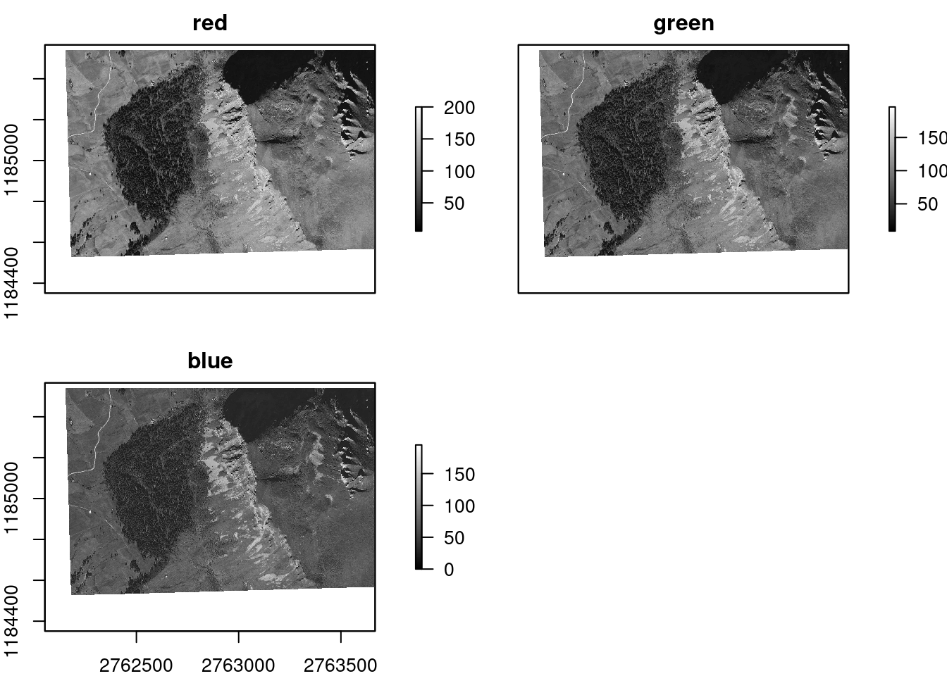
As you can see, the layers are not perfectly aligned horizontally. This is because we reprojected the data to the local LV-95 projection. To make sure everything is perfectly aligned, we can crop the bands to our aoi.
# Crop the layers to the aoi
sat <- crop(sat, aoi)

# Plot them again
plot(sat, col = gray(0:100/100), nrow = 1)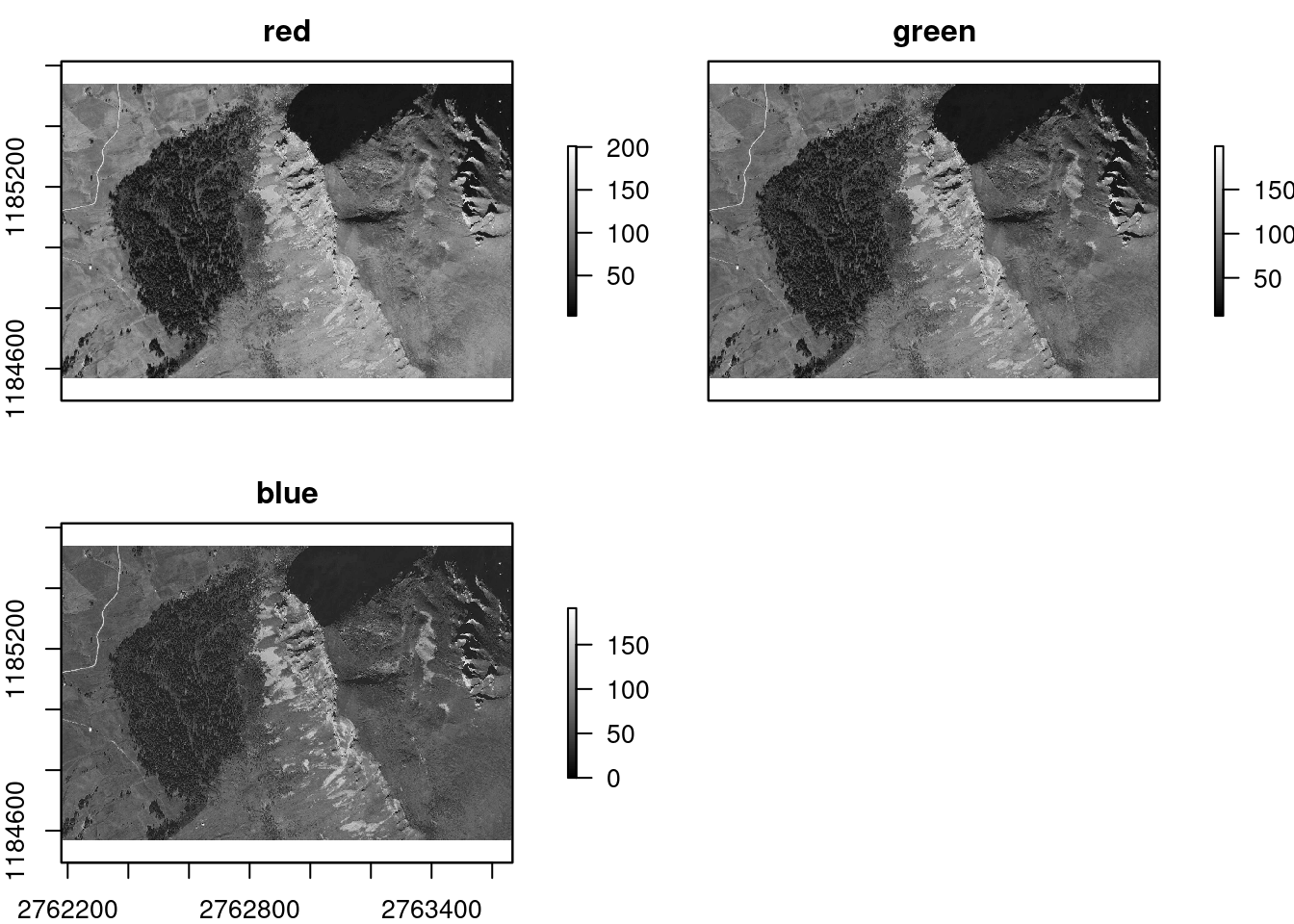
Plotting the Downloaded Imagery
Obvously we don’t want to plot the bands separately but want to combine them into a single RGB image. Here, I’ll show you how to achieve this using three different plotting engines.
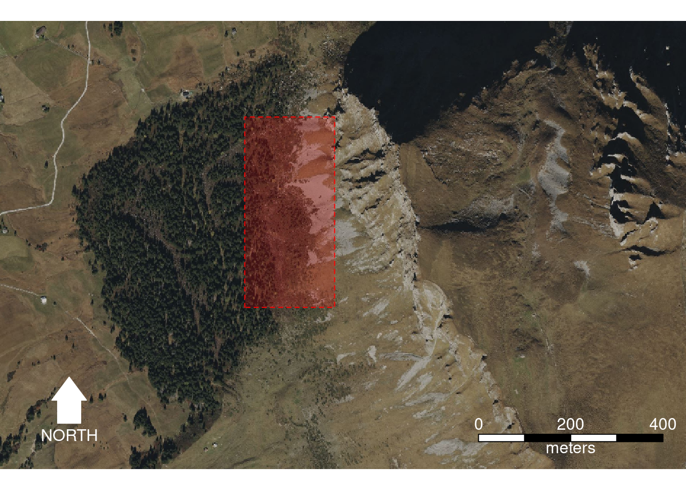
Using Base Plot
With R’s base plot we can plot RGB rasterlayers using the plotRGB() command.
This function takes the rasterstack and combines the layers into a color-image.
To make the plot look more professional and give some spatial reference, we can
also add a north arrow and a scale bar to the final image.
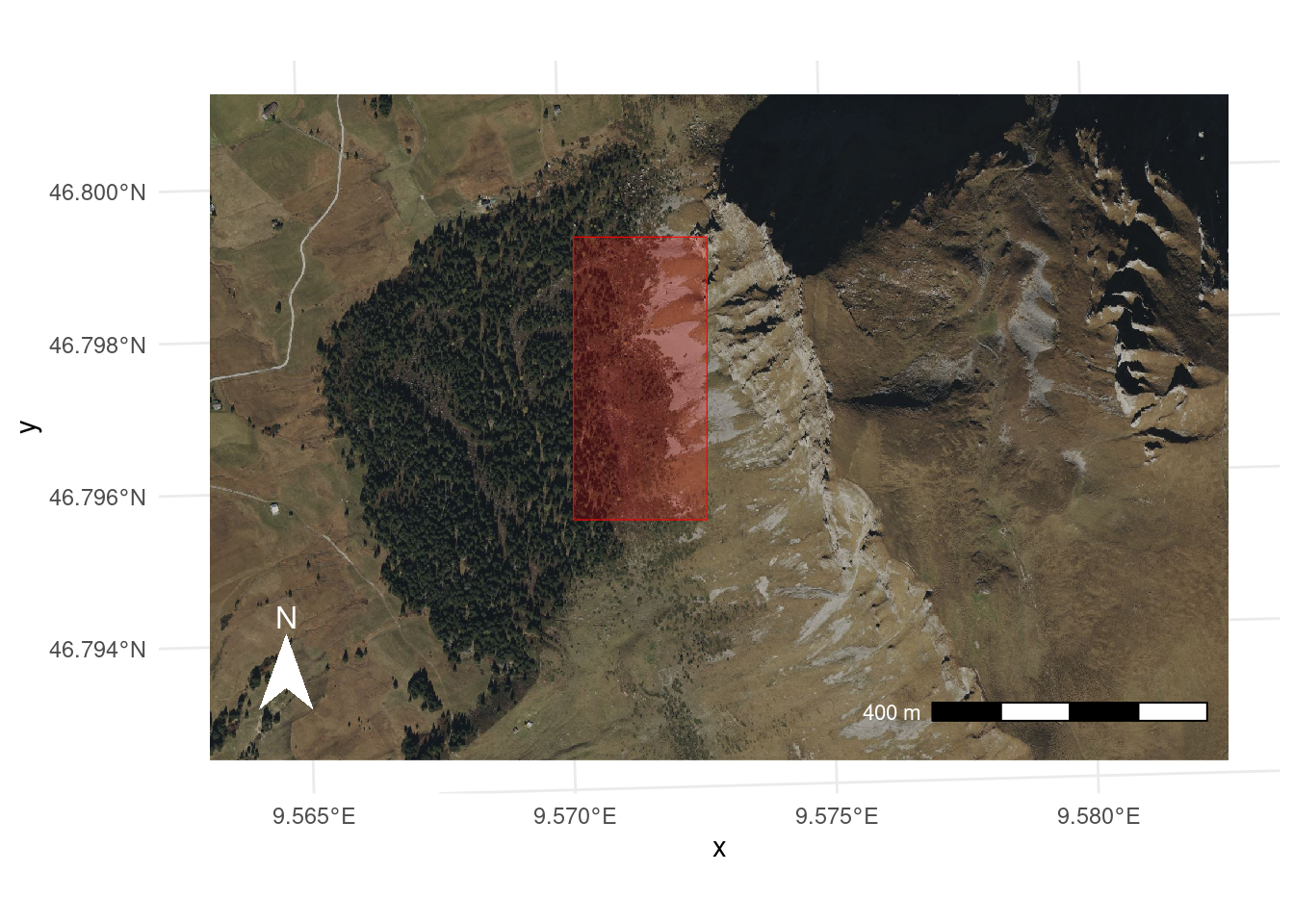
# Visualize the satellite image using R's base plot
plotRGB(sat, r = 1, g = 2, b = 3, axes = F)
plot(study_area, add = T, lty = 2, border = "red", col = adjustcolor("red", alpha.f = 0.2))
north.arrow(
    xb     = xmin(sat) + 150
  , yb     = ymin(sat) + 100
  , len    = 25
  , col    = "white"
  , border = "white"
  , tcol   = "white"
)
scalebar(
    type  = "bar"
  , xy    = c(xmax(sat) - 450 , ymin(sat) + 60)
  , d     = 400
  , divs  = 4
  , below = "meters"
  , col   = "white"
)
Using Ggplot
We can also plot our satellite data using the ggplot2 package. However,
instead of plotting the raster-stack directly, we first need to convert the
layers into a regular dataframe. This can easily be done using the
as.data.frame() function. Note that we specify xy = T to ensure that the
coordinates of each pixel in the rasters are retained.
# Convert the rasterstack to a regular dataframe
df <- as.data.frame(sat, xy = T)
head(df)
## x y red green blue
## 1 2762180 1185540 95 95 67
## 2 2762180 1185540 95 95 67
## 3 2762181 1185540 95 95 67
## 4 2762182 1185540 95 95 67
## 5 2762183 1185540 94 94 66
## 6 2762184 1185540 91 94 65We can then map the rgb values of each coordinate in ggplot as follows:
# Visualize the satellite image using ggplot
ggplot(df, aes(x = x, y = y, fill = rgb(red, green, blue, maxColorValue = 255))) +
  geom_raster() +
  scale_fill_identity() +
  coord_sf() +
  theme_minimal() +

  # Study area
  geom_sf(
      data        = st_as_sf(study_area)
    , inherit.aes = F
    , col         = "red"
    , fill        = "red"
    , alpha       = 0.2
  ) +

  # North arrow
  annotation_north_arrow(
      location = "bl"
    , pad_x    = unit(1, "cm")
    , pad_y    = unit(1, "cm")
    , style    = north_arrow_fancy_orienteering(
          fill      = c("white", "white")
        , line_col  = NA
        , text_col  = "white"
        , text_size = 12
      )
  ) +

  # Scalebar
  annotation_scale(
      location = "br"
    , pad_x    = unit(1, "cm")
    , pad_y    = unit(1, "cm")
    , text_col = "white"
  )
Using Tmap
One of my favorite packages to create pretty maps is called tmap. The syntax
of tmap is a bit unusual and takes some time to get used to but once learned,
tmap is a really powerful mapping tool. If you are not familiar with the
package, it is definitely worth checking out its
vignette.
Anyways, let’s plot our satellite imagery with tmap using the tm_shape() and
tm_rgb() functions.
# Visualize the satellite image using tmap
tm_shape(sat) +
    tm_rgb() +

  # Study area
  tm_shape(study_area) +
    tm_polygons(col = "red", alpha = 0.2, border.col = "red", border.alpha = 1) +

  # North arrow
  tm_compass(
      position   = c("left", "bottom")
    , text.color = "white"
    , color.dark = "white"
  ) +

  # Scalebar
  tm_scale_bar(
      position   = c("right", "bottom")
    , text.color = "white"
  ) +
  tm_graticules(lines = F)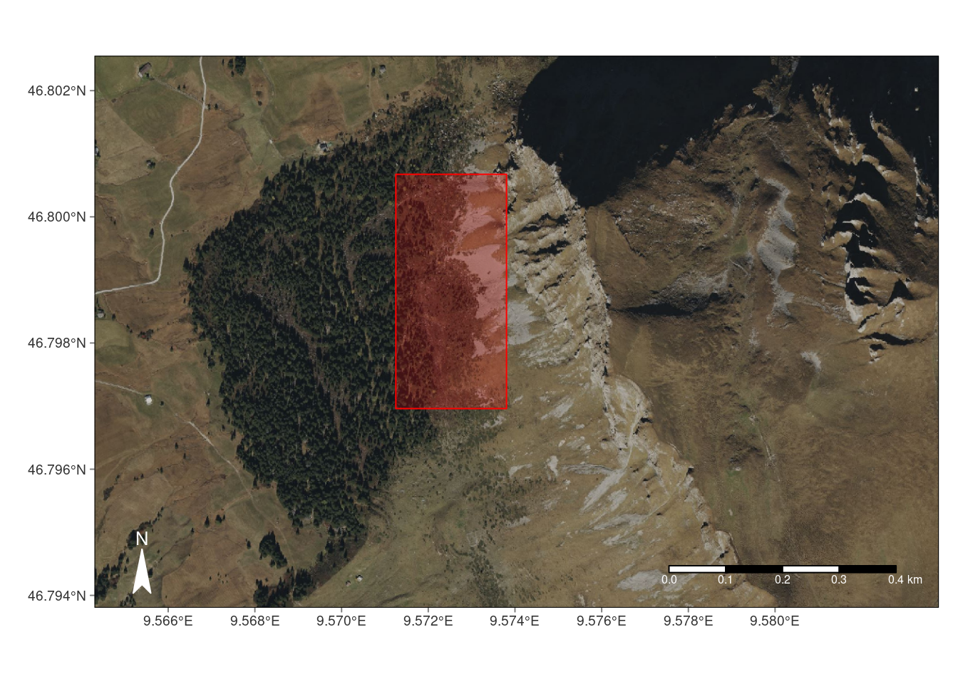
Summary
In this blog post we learned a relatively simple approach to download and visualize free satellite imagery from Microsoft Bing using R.
Session Information
## R version 4.1.2 (2021-11-01)
## Platform: x86_64-pc-linux-gnu (64-bit)
## Running under: Linux Mint 21.3
##
## Matrix products: default
## BLAS:   /usr/lib/x86_64-linux-gnu/blas/libblas.so.3.10.0
## LAPACK: /usr/lib/x86_64-linux-gnu/lapack/liblapack.so.3.10.0
##
## locale:
##  [1] LC_CTYPE=de_CH.UTF-8          LC_NUMERIC=C
##  [3] LC_TIME=de_CH.UTF-8           LC_COLLATE=de_CH.UTF-8
##  [5] LC_MONETARY=de_CH.UTF-8       LC_MESSAGES=de_CH.UTF-8
##  [7] LC_PAPER=de_CH.UTF-8          LC_NAME=de_CH.UTF-8
##  [9] LC_ADDRESS=de_CH.UTF-8        LC_TELEPHONE=de_CH.UTF-8
## [11] LC_MEASUREMENT=de_CH.UTF-8    LC_IDENTIFICATION=de_CH.UTF-8
##
## attached base packages:
## [1] stats     graphics  grDevices utils     datasets  methods   base
##
## other attached packages:
##  [1] tmap_3.3-3         ggspatial_1.1.9    sf_1.0-13          ggplot2_3.4.4
##  [5] GISTools_0.7-4     rgeos_0.6-3        MASS_7.3-55        RColorBrewer_1.1-3
##  [9] maptools_1.1-7     tmaptools_3.1-1    raster_3.6-20      sp_1.6-1
##
## loaded via a namespace (and not attached):
##  [1] sass_0.4.6          jsonlite_1.8.5      viridisLite_0.4.2
##  [4] bslib_0.5.0         highr_0.10          yaml_2.3.7
##  [7] OpenStreetMap_0.3.4 pillar_1.9.0        lattice_0.20-45
## [10] glue_1.6.2          digest_0.6.31       colorspace_2.1-0
## [13] htmltools_0.5.5     XML_3.99-0.14       pkgconfig_2.0.3
## [16] stars_0.6-1         s2_1.1.4            bookdown_0.34
## [19] scales_1.2.1        terra_1.7-74        tibble_3.2.1
## [22] proxy_0.4-27        generics_0.1.3      farver_2.1.1
## [25] cachem_1.0.8        withr_2.5.2         leafsync_0.1.0
## [28] cli_3.6.1           magrittr_2.0.3      evaluate_0.21
## [31] fansi_1.0.5         lwgeom_0.2-13       foreign_0.8-82
## [34] class_7.3-20        blogdown_1.17       tools_4.1.2
## [37] lifecycle_1.0.4     munsell_0.5.0       compiler_4.1.2
## [40] jquerylib_0.1.4     e1071_1.7-13        rlang_1.1.2
## [43] classInt_0.4-9      units_0.8-2         grid_4.1.2
## [46] dichromat_2.0-0.1   htmlwidgets_1.6.2   crosstalk_1.2.0
## [49] leafem_0.2.0        base64enc_0.1-3     rmarkdown_2.22
## [52] wk_0.7.3            gtable_0.3.3        codetools_0.2-18
## [55] abind_1.4-5         DBI_1.1.3           R6_2.5.1
## [58] knitr_1.43          dplyr_1.1.3         rgdal_1.6-6
## [61] fastmap_1.1.1       utf8_1.2.4          KernSmooth_2.23-20
## [64] rJava_1.0-6         parallel_4.1.2      Rcpp_1.0.11
## [67] vctrs_0.6.4         png_0.1-8           leaflet_2.2.0.9000
## [70] tidyselect_1.2.0    xfun_0.39