Introduction
When using a statistical model to predict an outcome of interest, we usually rely on point estimates, meaning that we use the coefficients’ estimated mean. However, in reality there is often considerable uncertainty such that point estimates can be rather inaccurate. Consequently, we are sometimes interested in the sensitivity of our predictions with respect to employed model parameters. This is exactly what we can examine using sensitivity analyses. That is, we predict or simulate the outcome of interest using different model parameters and check how varying parameters influences our results.
Coding a sensitivity analysis can be a bit of a challenge because it involves rigorous bookkeeping of used parameters and corresponding model outputs. It is therefore often worthwile to invest a bit of time and effort to create compartementalized code, so that we don’t need to copy and paste the same code over and over again. In addition, we want to avoid using loops, as loops tend to make things even more complicated.
In this blog post, I will show you my personal approach to quickly implement a sensitivity analysis in R. In principle, the approach consists of two parts. First, we write out a generalized function that allows us to predict the outcome of interest for a given set of parameters. Second, we apply the function repeatedly across different model parameters that we want to consider. For this, we heavily rely on the tidyverse package. In particular, we will make use of ‘tibbles’, which are tidyverse’s alternative to dataframes that allow to neatly store lists of lists. More on this later. But enough blabbing, let’s get started.
Model
For the purpose of this blog post, we will consider a simple matrix population model. The same workflow can of course be applied to any other modeling framework. Anyways, withouth going into too much detail, matrix population models are used by ecologists to project stage- or age-structured populations into the future using matrix algrebra. They require two basic ingredients: a transition matrix \(A\) and an initial population vector \(n_0\). While the transition matrix governs survival, fecundity, and transtions of the different classes, the initial population vector describes the number of individuals contained in each stage/age class at time zero. Once these two elements are known, one can predict or simulate the initial population into the future based on the dynamics dictated by the transition matrix using the following equation:
\[ n_{t + 1} = A * n_{t} \]
Here, we will assume a very basic two-stage population model with only juveniles (subscript \(j\)) and adults (subscript \(a\)), where juveniles develop into adults after one timestep. Moreover, we will assume that juvenile survival (\(S_j\)) depends on the temperature and that fecundity of adults (\(F_a\)) depends on the size of the population (i.e. adult survival is density dependent). Juvenile fecundity (\(F_j\)) is set to 0, and adult survival (\(S_a\)) is set to a probability of 0.9. Based on this knowledge, we can write out the transition matrix as follows:
\[ A = \begin{bmatrix} F_j = 0 & F_a(popsize) \\ S_j(temp) & S_a = 0.9 \\ \end{bmatrix} \]
Because we assume that \(F_a\) and \(S_j\) depend on other factors (the population size and temperature of the environment), we need to define functions that describe the functional forms of these relationships. Let us write two functions that make use of a linear-regression model and the inverse logit to transform predictions onto a range between 0 and 1. Note that we allow for non-linear functional forms by enabling second degree polynomials (i.e. \(x + x^2\)).
# Load required libraries
library(tidyverse)

# Define the inverse logit (sigmoid) function
invlogit <- function(x){1 / (1 + exp(-x))}

# Function that determines juvenile survival based on the current temperature
Sj <- function(temp, alpha, beta_1, beta_2){
  invlogit(alpha + beta_1 * temp + beta_2 * temp ** 2)
}

# Function that determines adult fecundity based on the current population size
Fa <- function(popsize, alpha, beta_1, beta_2){
  invlogit(alpha + beta_1 * popsize + beta_2 * popsize ** 2)
}
As you can see, we have not entered any specific values for alpha, beta_1, and beta_2 in the two funtions. This will allow us to later manipulate the functional forms of \(S_j\) and \(F_a\) to see how varying the parameters influences our model predictions. Using the functions it is now straight forward to plot the reaction curves for a given set of parameters under a given temperature and population size.
# Define the range of potential temperatures and population sizes
temprange <- c(-5:35)
poprange <- c(0:100)

# Visualize dependencies
par(mfrow = c(1, 2))
plot(Sj(temprange, -3, 0.3, -0.008) ~ temprange
  , col = "blue"
  , type = "l"
  , xlab = "Temperature (degrees Celsius)"
  , ylab = "Sj"
  , main = "Temperature Dependence"
  , las  = 1
)
plot(Fa(poprange, 3, -0.1, 0) ~ poprange
  , col = "blue"
  , type = "l"
  , xlab = "Population Size"
  , ylab = "Fa"
  , main = "Density Dependence"
  , las  = 1
)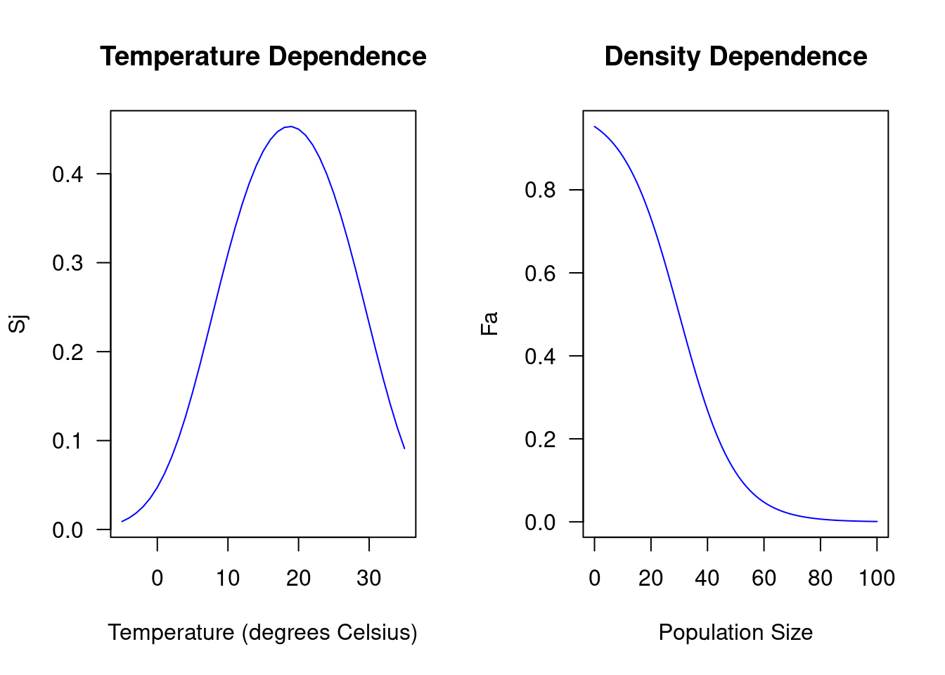
As you can see, with this set of parameters, juvenile survival (\(S_j\)) is
highest at around 20 degrees Celsius, whereas adult fecundity (\(F_a\)) is
highest when the population size is at its minimum. Thus, there is negative
density dependence, meaning that fecundity decreases as the population size
increases. In general, the transition matrix \(A\) will vary depending on the
temperature, the population size, and the parameters that define the functional
forms of \(S_j\) and \(F_a\). Now instead of manually defining the transition
matrix \(A\) for each desired combination of these variables, let’s write a
function createMat() that automatically generates the transition matrix \(A\)
for a given set of parameters and a given temperature and population size. Using
such a generic form of defining the matrix will later allow us to easily
manipulate the parameters that describe the functional forms of \(S_j\) and
\(F_j\). This also implies that the createMat() function needs to be able to
take those parameters as arguements.
# Function to generate the transition matrix for a given temperature, population
# size, and set of functional form parameters. This is probably the most crucial
# function!
createMat <- function(
    temp             # Temperature at a given time step
  , popsize          # Population size at a given time step
  , temp_alpha       # Intercept for temperature effect
  , temp_beta_1      # Slope one for temperature effect
  , temp_beta_2      # Slope two for temperature effect (squared effect)
  , popsize_alpha    # Intercept for population size effect
  , popsize_beta_1   # Slope one for population size effect
  , popsize_beta_2   # Slope one for population size effect (squared effect)
  ){
    fj <- 0
    sa <- 0.9
    fa <- Fa(popsize, popsize_alpha, popsize_beta_1, popsize_beta_2)
    sj <- Sj(temp, temp_alpha, temp_beta_1, temp_beta_2)
    A <- matrix(c(fj, fa, sj, sa), nrow = 2, byrow = T)
    return(A)
}
Let’s try out the function and see how we can generate a transition matrix for a given set of parameters and a given temperature and population size.
# Let's try if the function actually works. To see how the vital rates are
# affected by these numbers, try out different values.
createMat(
    temp           = 20
  , popsize        = 50
  , temp_alpha     = -3
  , temp_beta_1    = 0.3
  , temp_beta_2    = -0.008
  , popsize_alpha  = 3
  , popsize_beta_1 = -0.1
  , popsize_beta_2 = 0
)
## [,1] [,2]
## [1,] 0.000000 0.1192029
## [2,] 0.450166 0.9000000This is a quite powerful function! We can, for example, use it to compare the
transition matrices resulting under different assumptions. For instance, let’s
see how the transition matrix is affected when the population size increases.
For this, prepare a vector of different population sizes and use the lapply()
function to generate transition matrices for each of the values, assuming that
everything else remains constant.
# Define a set of different population sizes
poprange <- c(0, 50, 100)
# Create transition matrix for each of these population sizes
lapply(poprange, function(x){
createMat(
temp = 20
, popsize = x # Here the 0, 50, and 100 will go
, temp_alpha = -3
, temp_beta_1 = 0.3
, temp_beta_2 = -0.008
, popsize_alpha = 3
, popsize_beta_1 = -0.1
, popsize_beta_2 = 0
)
})## [[1]]
## [,1] [,2]
## [1,] 0.000000 0.9525741
## [2,] 0.450166 0.9000000
##
## [[2]]
##          [,1]      [,2]
## [1,] 0.000000 0.1192029
## [2,] 0.450166 0.9000000
##
## [[3]]
## [,1] [,2]
## [1,] 0.000000 0.0009110512
## [2,] 0.450166 0.9000000000As you can see, adult fecundity decreases from 0.95 to 0.11 and 0.0009 when as the population size increases, which is exactly what we expect given that there is density dependence.
Simulation Function
All that is left to do now is to run population projections under different
model parameters. In order to be able to quickly repeat our simulation multiple
times and for different parameters, we want to wrap our population projection
into a single function called simulation(). Given an initial population, a
vector of temperatures, and a set of model parameters (passed via the “…”),
the simulation() function will project population dynamics into the future.
# Simulation function to project our population into the future. Note that I'll
# use the "..." in order to pass the arguments needed by the createMat function,
# i.e. our parameter estimates for density and temperature
simulation <- function(pop, temp, ...){

  # Prepare empty matrix into which we will store the simulated data. Row one is
  # for juveniles, row two is for adults. Each column represents one timestep.
  # Note that the number of simulated iterations is determined by the length of
  # the "temperature" vector.
  population <- matrix(NA, nrow = 2, ncol = length(temp))

  # Put initial population into the first column
  population[, 1] <- pop

  # Loop through each timestep and project population dynamics
  for (i in 2:ncol(population)){

    # Update transition matrix based on temperature and population density
    A <- createMat(temp = temp[i], popsize = sum(population[, i - 1]), ...)

    # Project population one step into the future
    population[, i] <- A %*% population[, i - 1]
  }
  return(population)
}
Let us test if the function actually works. For this, we provide an initial population vector with 10 juveniles and 10 adults, and we randomly sample a time series of temperatures. Note that the length of this time series directly determines the number of iterations that we’re going to simulate! Finally, we specify a set of model parameters used for the simulation. We will later tweak these values.
# Test if the function works
simulation(
    pop            = c(10, 10)
  , temp           = rnorm(n = 5, mean = 20, sd = 5)
  , temp_alpha     = -3
  , temp_beta_1    = 0.3
  , temp_beta_2    = -0.008
  , popsize_alpha  = 3
  , popsize_beta_1 = -0.1
  , popsize_beta_2 = 0
)
## [,1] [,2] [,3] [,4] [,5]
## [1,] 10 7.310586 9.465035 9.536333 10.08021
## [2,] 10 13.088968 15.042423 17.814294 18.47994Great! This works as expected. The function returns a matrix where each column shows the number of juveniles and adults at a given point in time. Since we provided a temperature vector of length five, the number of simulated iterations is also equal to five.
Sensitivity Analysis
Now we are all settled for our sensitivity analysis and we can project our
population into the future using different parameters. This is where the power
of tibbles comes into play. For this, we first span a grid that contains all
combinations of parameters that we want to test for. This can easily be done
using the expand_grid() function. Moreover, we can use the function to specify
how many replicates of each combination we wish to run (this will allow us to
come up with bootstrap confidence intervals). Although we could now vary all six
parameters describing the functional forms of \(S_j\) and \(F_a\), (i.e.
\(\alpha_{temp}, \beta_{1, temp}, \beta_{2, temp}, \alpha_{popsize}, \beta_{1, popsize}, \beta_{2, popsize}\)), this will result in too many different outputs.
Hence, we are only going to vary \(\beta_{1, temp}\) and \(\beta_{1, popsize}\)
and we will repeat each simulation 100 times (i.e. 100 replicates). Note that
the expand_grid() automatically produces all unique combinations of parameters
and replicates.
# Specify the different treatment combinations, as well as the number of
# replicates. The function will then automatically generate all unique
# combinations.
design <- expand_grid(
    temp_beta_1    = c(0.2, 0.3, 0.4)
  , popsize_beta_1 = c(-0.1, -0.3, -0.5)
  , replicate      = 1:100
)
print(design, n = 5)
## # A tibble: 900 × 3
## temp_beta_1 popsize_beta_1 replicate
## <dbl> <dbl> <int>
## 1 0.2 -0.1 1
## 2 0.2 -0.1 2
## 3 0.2 -0.1 3
## 4 0.2 -0.1 4
## 5 0.2 -0.1 5
## # ℹ 895 more rowsIt is now tempting to use a “for-loop” to go through each row and apply our
simulation() function. However, for-loops are a nightmare for bookkeeping. In
addition, we want to make use of these fancy “tibble” dataframes. Thus, I prefer
to use the lapply() function, which directly returns a list comprising the
results of each simulation. This allows us to conveniently store the resulting
output directly in a new column the “design” tibble, such that we readily know
which simulation belongs to which set of parameters.
# Run our simulation for each row of the design dataframe
design$Simulation <- lapply(1:nrow(design), function(x){

  # Run simulation
  population <- simulation(
      pop            = c(10, 10)                         # 10 juveniles, 10 adults
    , temp           = rnorm(n = 100, mean = 20, sd = 5) # Random temperatures
    , temp_alpha     = -3
    , temp_beta_1    = design$temp_beta_1[x]
    , temp_beta_2    = -0.008
    , popsize_alpha  = 3
    , popsize_beta_1 = design$popsize_beta_1[x]
    , popsize_beta_2 = 0
  )

  # Tidy the data (cast matrix to dataframe and convert it from wide to long format)
  population <- as.data.frame(population)
  population <- cbind(c("Juveniles", "Adults"), population)
  names(population) <- c("Stage", 1:(ncol(population) - 1))
  population <- gather(population
    , key   = "Year"
    , value = "Count"
    , 2:ncol(population)
  )

  # Coerce the Year column from character to numeric
  population$Year <- as.numeric(population$Year)

  # Return the simulated and tidied data
  return(population)
})

# Let's take a look at the produced object
print(design, n = 5)
## # A tibble: 900 × 4
## temp_beta_1 popsize_beta_1 replicate Simulation
## <dbl> <dbl> <int> <list>
## 1 0.2 -0.1 1 <df [200 × 3]>
## 2 0.2 -0.1 2 <df [200 × 3]>
## 3 0.2 -0.1 3 <df [200 × 3]>
## 4 0.2 -0.1 4 <df [200 × 3]>
## 5 0.2 -0.1 5 <df [200 × 3]>
## # ℹ 895 more rowsAs you can see, each row of the “design” tibble now contains the simulated data belonging to the respective parameter set. This makes it very easy to keep track of the different simulations and the employed parameters. Moreover, we can subset and access simulations as we wish. For this, we simply subset the data according to our likings, and unnest the remaining rows (i.e. un-collapse the stored dataframes).
# Take a subset and unnest
design %>%
  subset(temp_beta_1 == 0.2) %>%
  unnest(Simulation)
## # A tibble: 60,000 × 6
## temp_beta_1 popsize_beta_1 replicate Stage Year Count
## <dbl> <dbl> <int> <chr> <dbl> <dbl>
## 1 0.2 -0.1 1 Juveniles 1 10
## 2 0.2 -0.1 1 Adults 1 10
## 3 0.2 -0.1 1 Juveniles 2 7.31
## 4 0.2 -0.1 1 Adults 2 10.1
## 5 0.2 -0.1 1 Juveniles 3 7.89
## 6 0.2 -0.1 1 Adults 3 9.54
## 7 0.2 -0.1 1 Juveniles 4 7.43
## 8 0.2 -0.1 1 Adults 4 8.78
## 9 0.2 -0.1 1 Juveniles 5 7.02
## 10 0.2 -0.1 1 Adults 5 8.23
## # ℹ 59,990 more rows# Take a subset and unnest
design %>%
subset(temp_beta_1 == 0.2 & popsize_beta_1 == -0.5) %>%
unnest(Simulation)## # A tibble: 20,000 × 6
## temp_beta_1 popsize_beta_1 replicate Stage Year Count
## <dbl> <dbl> <int> <chr> <dbl> <dbl>
## 1 0.2 -0.5 1 Juveniles 1 10
## 2 0.2 -0.5 1 Adults 1 10
## 3 0.2 -0.5 1 Juveniles 2 0.00911
## 4 0.2 -0.5 1 Adults 2 9.84
## 5 0.2 -0.5 1 Juveniles 3 1.25
## 6 0.2 -0.5 1 Adults 3 8.86
## 7 0.2 -0.5 1 Juveniles 4 1.01
## 8 0.2 -0.5 1 Adults 4 8.12
## 9 0.2 -0.5 1 Juveniles 5 1.41
## 10 0.2 -0.5 1 Adults 5 7.41
## # ℹ 19,990 more rowsVisualization
Finally, we want to visualize the simulated data using ggplot to get an idea how the number of juveniles and adults develops over time under the different parameters. For this, we unnest all the data, thereby creating single big dataframe.
# Let's unnest all data and visualize our simulations
dat <- unnest(design, Simulation)

# Check it
head(dat)
## # A tibble: 6 × 6
## temp_beta_1 popsize_beta_1 replicate Stage Year Count
## <dbl> <dbl> <int> <chr> <dbl> <dbl>
## 1 0.2 -0.1 1 Juveniles 1 10
## 2 0.2 -0.1 1 Adults 1 10
## 3 0.2 -0.1 1 Juveniles 2 7.31
## 4 0.2 -0.1 1 Adults 2 10.1
## 5 0.2 -0.1 1 Juveniles 3 7.89
## 6 0.2 -0.1 1 Adults 3 9.54Once unnested, we can calculate summary statistics across replicates for each specific parameter combination. Here, we calculate the mean and the 2.5% and 97.5% percentiles. We can later use those to generate confidence-bands.
# Average counts of juveniles and adults across replicates and calculate
# prediction intervals
tallied <- dat %>%
  group_by(temp_beta_1, popsize_beta_1, Stage, Year) %>%
  summarize(
      Lower   = quantile(Count, 0.025)
    , Upper   = quantile(Count, 0.975)
    , Count   = mean(Count)
    , .groups = "drop"
  )

# Check it
head(tallied)
## # A tibble: 6 × 7
## temp_beta_1 popsize_beta_1 Stage Year Lower Upper Count
## <dbl> <dbl> <chr> <dbl> <dbl> <dbl> <dbl>
## 1 0.2 -0.5 Adults 1 10 10 10
## 2 0.2 -0.5 Adults 2 9.13 10.5 9.94
## 3 0.2 -0.5 Adults 3 8.21 9.43 8.95
## 4 0.2 -0.5 Adults 4 7.61 8.60 8.18
## 5 0.2 -0.5 Adults 5 6.96 7.86 7.45
## 6 0.2 -0.5 Adults 6 6.35 7.24 6.83Finally, we can plot the population dynamics for each of the parameter combinations and add the confidence bands previously calculated.
# Plot
ggplot(tallied, aes(x = Year, y = Count, color = Stage, fill = Stage)) +
  geom_ribbon(aes(ymin = Lower, ymax = Upper), alpha = 0.2, lwd = 0.2) +
  geom_line(size = 0.1) +
  facet_wrap(~ temp_beta_1 + popsize_beta_1
    , labeller = label_both
    , scales   = "free"
  ) +
  theme_classic() +
  theme(legend.position = "bottom")
## Warning: Using `size` aesthetic for lines was deprecated in ggplot2 3.4.0.
## ℹ Please use `linewidth` instead.
## This warning is displayed once every 8 hours.
## Call `lifecycle::last_lifecycle_warnings()` to see where this warning was
## generated.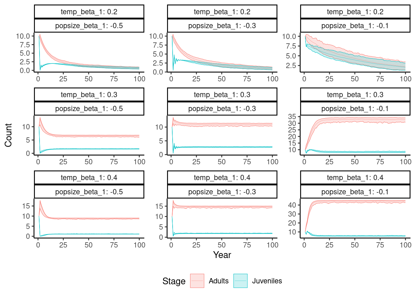
And there you have it. A nice sensitivity analysis with relatively few lines of code.
Summary
In this post we conducted a relatively simple sensitivity analysis of a matrix
population model. For this, we first wrote a simulation() function which
automated model predictions for a given set of parameters. Afterwards, we
defined a design matrix comprising all combinations of parameters for which we
wanted to run the simulation. Finally, we ran the simulation for each set of
parameters and stored the output neatly in a tibble and plotted the results
using ggplot.
Session Information
## R version 4.1.2 (2021-11-01)
## Platform: x86_64-pc-linux-gnu (64-bit)
## Running under: Linux Mint 21.3
##
## Matrix products: default
## BLAS:   /usr/lib/x86_64-linux-gnu/blas/libblas.so.3.10.0
## LAPACK: /usr/lib/x86_64-linux-gnu/lapack/liblapack.so.3.10.0
##
## locale:
##  [1] LC_CTYPE=de_CH.UTF-8       LC_NUMERIC=C
##  [3] LC_TIME=de_CH.UTF-8        LC_COLLATE=de_CH.UTF-8
##  [5] LC_MONETARY=de_CH.UTF-8    LC_MESSAGES=de_CH.UTF-8
##  [7] LC_PAPER=de_CH.UTF-8       LC_NAME=C
##  [9] LC_ADDRESS=C               LC_TELEPHONE=C
## [11] LC_MEASUREMENT=de_CH.UTF-8 LC_IDENTIFICATION=C
##
## attached base packages:
## [1] stats     graphics  grDevices utils     datasets  methods   base
##
## other attached packages:
##  [1] lubridate_1.9.3 forcats_1.0.0   stringr_1.5.1   dplyr_1.1.3
##  [5] purrr_1.0.2     readr_2.1.4     tidyr_1.3.0     tibble_3.2.1
##  [9] ggplot2_3.4.4   tidyverse_2.0.0
##
## loaded via a namespace (and not attached):
##  [1] highr_0.10       bslib_0.5.0      compiler_4.1.2   pillar_1.9.0
##  [5] jquerylib_0.1.4  tools_4.1.2      digest_0.6.31    timechange_0.2.0
##  [9] jsonlite_1.8.5   evaluate_0.21    lifecycle_1.0.4  gtable_0.3.3
## [13] pkgconfig_2.0.3  rlang_1.1.2      cli_3.6.1        yaml_2.3.7
## [17] blogdown_1.17    xfun_0.39        fastmap_1.1.1    withr_2.5.2
## [21] knitr_1.43       hms_1.1.3        generics_0.1.3   sass_0.4.6
## [25] vctrs_0.6.4      grid_4.1.2       tidyselect_1.2.0 glue_1.6.2
## [29] R6_2.5.1         fansi_1.0.5      rmarkdown_2.22   bookdown_0.34
## [33] farver_2.1.1     tzdb_0.4.0       magrittr_2.0.3   scales_1.2.1
## [37] htmltools_0.5.5  colorspace_2.1-0 labeling_0.4.2   utf8_1.2.4
## [41] stringi_1.8.1    munsell_0.5.0    cachem_1.0.8     crayon_1.5.2