What is Scaling
When we run a regression model, we typically scale our covariates prior to including them in the model. We usually do this out of habit, without really thinking much about happens in the background. In this document, I will try to explain the main reasons for scaling and how scaling influences the interpretation of the model coefficients. Finally, I will show you how you can “back-transform” the coefficients from a linear model in which covariates were scaled into the unscaled world.
Now before we dive into the details, let’s clarify what I really mean by
“scaling”. When I talk about scaling, I actually refer to “standardizing” a
covariate to a mean of zero and a standard deviation of one. Standardization is
achieved by subtracting the covariate’s mean \(\mu_x\) and dividing by its
standard deviation \(\sigma_x\). In R, this can conveniently be achieved using
the built in function scale(), which by default applies the following formula:
\[ X_{scaled} = \frac{X - \mu_x}{\sigma_x} \]
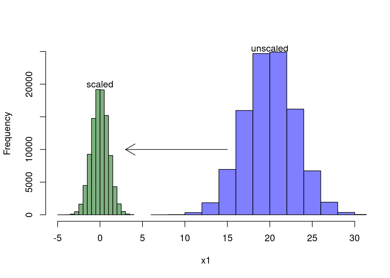
To understand how the scale() function works, take a look at the two
histograms below. The blue histogram shows the distribution of the original
covariate \(X\), whereas the green histogram depicts the distribution of \(X_1\)
after we scaled it with the scale() function. As you can see, scaling moves
the distribution to the left and makes it much narrower. In fact, it moves the
distribution such that it’s mean is at zero and it squeezes the distribution so
that the standard deviation is equals one. Note, however, that scaling doesn’t
affect the skewness of the distribution.
The idea is then to use the scaled covariate \(X_{scaled}\) instead of the unscaled covariate \(X\) in our regression model. Importantly though, including a scaled covariate instead of its unscaled counterpart does not affect the mathematical structure the final model, which is also the reason why we can easily go back and forth between scaled and unscaled model coefficients. We can actually proof that the mathematical formula of the model remains the same:
\[ \begin{aligned} Y &= \beta_0 + \beta_1 \frac{(X_1 - \mu_1)}{\sigma_1}\\ &= \underbrace{\beta_0 - \beta_1 \frac{\mu_1}{\sigma_1}}_{\beta_0'} + \underbrace{\beta_1\frac{X_1}{\sigma_1}}_{\beta_1' X_1}\\ &= \beta_0' + \beta_1'X_1 \end{aligned} \]
Instead of influencing the mathematical structure of the model, scaling will affect model coefficients (from \(\beta_0\) to \(\beta_0'\) and from \(\beta_1\) to \(\beta_1'\)). This is essentially because covariates are on different scales, which also implies that we need to interpret the \(\beta\)s differently. We’ll talk about this a bit later. Despite the fact that the model remains formally the same, scaling can be beneficial in some cases.
Why to Scale
There are several reasons why you might want to scale your covariates prior to including them in a regression model. Let’s go through them individually:
To ease the interpretation of the intercept: If you don’t scale your covariates, the intercept of your model is interpreted as the expected value of your outcome variable \(Y\) when all covariates are set to 0. In many cases, covariates set to 0 make little sense (e.g. if you consider age or height of a person as covariates) and so the intercept is rather meaningless in that case. When all of your covariates are scaled, on the other hand, the intercept of your model becomes a meaningful value. It can be interpreted as the expected value of Y when all covariates are at their means (e.g. the expected weight of a person that is at average age and height). This becomes particularly helpful if your model contains interaction terms, which we will see later.
To bring coefficients “closer together”: Sometimes your covariates will be on very different scales; some on a very large scale, others on a small scale. This can result in regression coefficients that are very dissimilar (some extremely small, some very large) and therefore much more difficult to interpret. Once covariates are scaled, this will no longer be an issue as covariates are essentially “scale free”.
To help with convergence issues: Some models use gradient descent algorithms to iteratively approach the maximul likelihood estimates of the desired regression coefficients. Scaling of covariates can substantially increase the efficiency of such algorithms and therefore mitigate convergence issues.
To reduce issues of collinearity: Quite often you will be interested in interactions between your covariates. Unfortunately, creating an interaction term results in high collinearity between main effects and their respective interactions. However, if you scale your variables prior to forming their interactions, you can usually prevent this issue. Let’s illustrate this with an example:
# Simulate two covariates
x1 <- rnorm(10000, 5, 2)
x2 <- rnorm(10000, 15, 2)

# Scale them
x1_scaled <- scale(x1)
x2_scaled <- scale(x2)

# Check for correlation of x1 with the interaction term for x1 and x2
as.vector(cor(x1, x1 * x2))
## [1] 0.9398006# Correlation becomes much smaller if we scale covariates
as.vector(cor(x1_scaled, x1_scaled * x2_scaled))## [1] 0.02327099# Check for correlation of x2 with the interaction term for x1 and x2
as.vector(cor(x2, x1 * x2))## [1] 0.3248103# Correlation becomes much smaller if we scale covariates
as.vector(cor(x2_scaled, x1_scaled * x2_scaled))## [1] 0.007118844I hope that by now you are convinced that scaling is a good thing. But let’s also look at some more complicated matters. More specifically, let’s evaluate how scaling influences the interpretation of interactions and how we can back-transform model coefficients obtained through scaled covariates.
A Note on Interactions
Models containing interaction terms can be incredibly challenging to interpret, especially if covariates are not scaled. To motivate this, let’s mathematically write down a model that contains interactions. Mathematically, we can represent an interaction between two continuous covariates in a linear model as follows:
\[ \begin{aligned} Y &= \beta_0 + \beta_1 X_1 + \beta_2 X_2 + \beta_3 X_1 X_2 \\ \end{aligned} \]
That is, in addition to the fixed effects \(\beta_1 X_1\) and \(\beta_2 X_2\), the linear model now also includes the product of the two covariates (in his case \(X_1\) and \(X_2\)), which is called interaction term \(\beta_3 X_1 X_2\). But how does this affect our interpretation of the \(\beta\)’s? In a model with interaction terms, the regression coefficients \(\beta_1\) and \(\beta_2\) represent conditional relationships, meaning that the influence of \(X_1\) on \(Y\) depends on the value of \(X_2\) and vice versa. For instance, if \(X_2 = 0\) our model simplifies to:
\[ \begin{aligned} Y &= \beta_0 + \beta_1 X_1 + \beta_2 * 0 + \beta_3 X_1 * 0 \\ &= \beta_0 + \beta_1 X_1 \end{aligned} \]
Hence, if \(X_2 = 0\), a one unit increase in \(X_1\) results in a \(\beta_1\) increase in \(Y\). Stated differently, when \(X_2 = 0\), then \(\beta_1\) indicates how a one unit increase in \(X_1\) effects \(Y\). However, in case we have \(X_2 = 2\), the model turns into:
\[ \begin{aligned} Y &= \beta_0 + \beta_1 X_1 + \beta_2 * 2 + \beta_3 X_1 * 2 \\ &= \beta_0 + X_1(\beta_1 + 2\beta_3) + 2 * \beta_2 \end{aligned} \]
In this case, a one unit increase in \(X_1\) results in a \(\beta_1 + 2\beta_3\) unit increase in \(Y\). As we can see, unless 0 represents a reasonable covariate value, we can’t meaningfully interpret the main effect estimators (i.e. \(\beta_1\) and \(\beta_2\)). But how does this change once we scale our covariates?
Initially, I have been struggling to understand how to properly scale
interactions and how scaling influences the interpretation of our model
estimates. In particular, I was confused about the differences between
scale(x1):scale(x2) and scale(x1:x2). In the first case, we scale the
covariates prior to forming their product. In the second case, we first form the
product (i.e. the interaction) and only scale the product afterwards. I used to
follow the first approach but I was getting insecure when I found that Ben
Bolker applied the second approach in a
post
on stackoverflow.
Besides this, I was also getting sceptical that scale(x1):scale(x2) would mess
up the “direction” of effects. For example, let’s assume that we measured two
covariates that are always positive. Without scaling, the interaction of two
high values will always be high (e.g. \(5 * 5 = 25\)), whereas the interaction
of two low values will always be low (\(0.5 * 0.5 = 0.25\)). However, once we
scale the two covariates this logic no longer applies. When scaled, both
covariates also cover negative values. As such, the interaction of two low
values (\(-5 * -5 = 25\)) can be the same as the interaction of two high values
(\(5 * 5 = 25\)). Similarly, two very different combinations can result in the
same interaction (\(-5 * 5 = -25\) and \(5 * -5 = -25\)). This may seem
confusing as we can suddenly no longer differentiate between high and low
covariate values based on the value of the interaction. However, this
differentiation is not the point of interactions. The point of interactions is
to see if joint extremes of the two covariates explains variability in our
outcome. In fact, when we scale our covariates prior to forming the interaction,
the interaction term becomes the index of how deviant the joint combination of
the two covariates is. This is exactly what we want. Consequently, I would
advise to go for the first approach and use scale(x1):scale(x2).
A second reason to opt for scale(x1):scale(x2) is the fact that scale(x1:x2)
introduces substantial collinearity among covariates, whereas using
scale(x1):scale(x2) effectively mitigates this risk. We can exemplify this as
follows:
# Simulate two covariates
x1 <- rnorm(10000, 5, 2)
x2 <- rnorm(10000, 15, 2)

  # Scale all of the variables
x1_scaled <- scale(x1)
x2_scaled <- scale(x2)
x1x2_scaled <- scale(x1 * x2)

# Check for correlation with interaction term
as.vector(cor(x1, x1 * x2))
## [1] 0.9419914as.vector(cor(x1_scaled, x1_scaled * x2_scaled))## [1] -0.002424096as.vector(cor(x1_scaled, x1x2_scaled))## [1] 0.9419914Consequently, you should always scale your covariates prior to forming their interactions.
The cool thing is, once the covariates are scaled, interpretation of model coefficients becomes much easier. For instance, \(\beta_1\) now indicates the effect of a one unit increase of \(X_1\) on \(Y\) when \(X_2\) (unscaled) is at its average (instead of at 0). Similarly, \(\beta_2\) indicates the effect of a one unit increase of \(X_2\) on \(Y\) when \(X_1\) (unscaled) is at its average. Consequently, scaling the covariates allows you to interpret the main effects \(\beta_1\) and \(\beta_2\) for more realistic values of \(X_1\) and \(X_2\). In addition, the intercept can now be interpreted as the expected value of \(Y\) when all other covariates are at their means (instead of 0). Again, it is important to understand that the model itself and its predictions remain the same. Scaling only influences the way in which we can interpret the model coefficients.
How to Backtransform Model Coefficients
In some cases, you may want to be able to convert your model output from the scaled world back into the unscaled world. This could be the case when you only scaled because you had convergence issues, but actually prefer to report your results on the unscaled covariate. Here, I want to show how you can *achieve this for two different cases.
Case I: The model contains no interactions:
\(Y = \beta_0 + \beta_1 X_{1, scaled} + \beta_2 X_{2, scaled}\)
Case II: The model contains interactions of scaled covariates:
\(Y = \beta_0 + \beta_1 X_{1, scaled} +\) \(\beta_2 X_{2, scaled} + \beta_3 X_{1, scaled} X_{2, scaled}\)
For each case, we’ll start by writing out the formula of the original, unscaled model. We then scale the covariates and try to rearrange everything so that we can describe the relationshipt between the coefficients from the scaled and unscaled model.
Case I: Unscale a Model without Interactions
The Math
Let’s write out our basic model and do some rearrangements to see the relationshipt between the coefficients from the scaled model (\(\beta'\)) and the coefficients of the unscaled model (\(\beta\)).
\[ \begin{aligned} Y &= \beta_0 + \beta_1 X_1 + \beta_2 X_2 \\ &= \beta_0' + \beta_1' \frac{X_1 - \mu_1}{\sigma_1} + \beta_2' \frac{X_2 - \mu_2}{\sigma_2} \\ &= \underbrace{ \beta_0' - \beta_1'\frac{\mu_1}{\sigma_1} - \beta_2'\frac{\mu_2}{\sigma_2} }_{\beta_0} + \underbrace{\beta_1'\frac{X_1}{\sigma_1}}_{\beta_1X_1} + \underbrace{\beta_2'\frac{X_2}{\sigma_2}}_{\beta_2X_2} \\ \end{aligned} \]
Hence, we can rewrite the model coefficients as follows:
\[ \beta_0 = \beta_0' - \beta_1'\frac{\mu_1}{\sigma_1} - \beta_2'\frac{\mu_2}{\sigma_2} \qquad \beta_1 = \frac{\beta_1'}{\sigma_1} \qquad \beta_2 = \frac{\beta_2'}{\sigma_2} \]
We can generalize this to a model with many more covariates:
\[ \beta_0 = \beta_0' - \sum_i\beta_i'\frac{\mu_i}{\sigma_i} \qquad \beta_i = \frac{\beta_i'}{\sigma_i} \]
Example
Let’s proof that this actually works using some simulated data.
# Simulate some data without interactions
n <- 1e5
x1 <- rnorm(n, mean = 5, sd = 2)
x2 <- rnorm(n, mean = -2, sd = 0.2)
e <- rnorm(n, mean = 0, sd = 1)
y <- 1 + 2 * x1 + 3 * x2 + e
dat <- data.frame(y, x1, x2)

# Run a model without scaling and extract the model coefficients
mod1 <- lm(y ~ x1 + x2, data = dat)
coefs1 <- coef(mod1)

# Run a model with scaling and extract the model coefficients
mod2 <- lm(y ~ scale(x1) + scale(x2), data = dat)
coefs2 <- coef(mod2)

# Try to backtransform the coefficients from the scaled model
# Intercept
coefs1[1]
## (Intercept)
## 1.011663coefs2[1] - coefs2[2] * mean(x1) / sd(x1) - coefs2[3] * mean(x2) / sd(x2)## (Intercept)
## 1.011663# Coefficient for x1
coefs1[2]## x1
## 1.999911coefs2[2] / sd(x1)## scale(x1)
## 1.999911# Coefficient for x2
coefs1[3]## x2
## 3.006133coefs2[3] / sd(x2)## scale(x2)
## 3.006133Case II: Unscale a Model with an Interaction of Scaled Covariates
The Math
Again, let’s start by writing out the unscaled model and work our way through to get the relationship between the model coefficients of the unscaled and scaled covariates.
\[ \begin{aligned} Y &= \beta_0 + \beta_1 X_1 + \beta_2 X_2 + \beta_3 X_1 X_2\\ &= \beta_0' + \beta_1' \frac{X_1 - \mu_1}{\sigma_1} + \beta_2' \frac{X_2 - \mu_1}{\sigma_2} + \beta_3' \left(\frac{X_1 - \mu_1}{\sigma_1}\right) \left(\frac{X_2 - \mu_2}{\sigma_2}\right) \\ &= \beta_0' + \beta_1' \frac{X_1 - \mu_1}{\sigma_1} + \beta_2' \frac{X_2 - \mu_2}{\sigma_2} + \beta_3' \frac{X_1 X_2 - X_1 \mu_2 - X_2 \mu_1 + \mu_1 \mu_2}{\sigma_1 \sigma_2} \\ &= \underbrace{\beta_0' - \beta_1' \frac{\mu_1}{\sigma_1} - \beta_2' \frac{\mu_2}{\sigma_2} + \beta_3' \frac{\mu_1 \mu_2}{\sigma_1 \sigma_2}}_{\beta_0} + \beta_1' \frac{X_1}{\sigma_1} + \beta_2' \frac{X_2}{\sigma_2} + \beta_3' \frac{X_1 X_2 - X_1 \mu_2 - X_2 \mu_1}{\sigma_1 \sigma_2} \\ &= \beta_0 + \beta_1' \frac{X_1}{\sigma_1} - \beta_3' \frac{X_1 \mu_2}{\sigma_1 \sigma_2} + \beta_2' \frac{X_2}{\sigma_2} - \beta_3' \frac{X_2 \mu_1}{\sigma_1 \sigma_2} + \beta_3' \frac{X_1 X_2}{\sigma_1 \sigma_2} \\ &= \beta_0 + \underbrace{ \left(\frac{\beta_1'}{\sigma_1} - \frac{\beta_3' \mu_2}{\sigma_1 \sigma_2}\right) }_{\beta_1} X_1 + \underbrace{ \left(\frac{\beta_2'}{\sigma_2} - \frac{\beta_3' \mu_1}{\sigma_1 \sigma_2}\right) }_{\beta_2} X_2 + \underbrace{\frac{\beta_3'}{\sigma_1 \sigma_2}}_{\beta_3} X_1 X_2\\ \end{aligned} \]
Hence, we can rewrite the model coefficients as follows:
\[ \beta_0 = \beta_0' - \beta_1'\frac{\mu_1}{\sigma_1} - \beta_2'\frac{\mu_2}{\sigma_2} + \beta_3'\frac{\mu_1 \mu_2}{\sigma_1 \sigma_2} \qquad \beta_1 = \frac{\beta_1'}{\sigma_1} - \frac{\beta_3' \mu_2}{\sigma_1 \sigma_2} \qquad \beta_2 = \frac{\beta_2'}{\sigma_2} - \frac{\beta_3' \mu_1}{\sigma_1 \sigma_2} \qquad \beta_3 = \frac{\beta_3'}{\sigma_1 \sigma_2} \]
Example
Let’s proof that this actually works using some simulated data.
# Simulate some data with an interaction
n <- 1e5
x1 <- rnorm(n, mean = 5, sd = 2)
x2 <- rnorm(n, mean = -2, sd = 0.2)
e <- rnorm(n, mean = 0, sd = 1)
y <- 1 + 2 * x1 + 3 * x2 + 0.5 * x1 * x2 + e
dat <- data.frame(y, x1, x2)

# Run a model without scaling and extract the model coefficients
mod1 <- lm(y ~ x1 + x2 + x1:x2, data = dat)
coefs1 <- coef(mod1)

# Run a model with scaling and extract the model coefficients
mod2 <- lm(y ~ scale(x1) + scale(x2) + scale(x1):scale(x2), data = dat)
coefs2 <- coef(mod2)

# Try to backtransform the coefficients from the scaled model
# Intercept
coefs1[1]
## (Intercept)
## 0.97524coefs2[1] - coefs2[2] * mean(x1) / sd(x1) - coefs2[3] * mean(x2) / sd(x2) +
coefs2[4] * mean(x1) * mean(x2) / (sd(x1) * sd(x2))## (Intercept)
## 0.97524# Coefficient for x1
coefs1[2]## x1
## 2.003916coefs2[2] / sd(x1) - coefs2[4] * mean(x2) / (sd(x1) * sd(x2))## scale(x1)
## 2.003916# Coefficient for x2
coefs1[3]## x2
## 2.976788coefs2[3] / sd(x2) - coefs2[4] * mean(x1) / (sd(x1) * sd(x2))## scale(x2)
## 2.976788# Coefficient for x1:x2
coefs1[4]## x1:x2
## 0.5035732coefs2[4] / (sd(x1) * sd(x2))## scale(x1):scale(x2)
## 0.5035732Great! It looks like our mathematics worked out and we are indeed able to “backtransform” our model relatively easily. I hope that with this blog post I could clarify the reasons behind scaling and how it actually works in detail. If you’re interested, you can find some additional material and reading below.
Further Reading
- The why and when of scaling/standardizing I: (https://www.goldsteinepi.com/blog/thewhyandwhenofcenteringcontinuouspredictorsinregressionmodeling/index.html)
- The why and when of scaling/standardizing II: (https://stats.stackexchange.com/questions/29781/when-conducting-multiple-regression-when-should-you-center-your-predictor-varia)
- The why and when of scaling/standardizing III: (https://stats.stackexchange.com/questions/19216/variables-are-often-adjusted-e-g-standardised-before-making-a-model-when-is)
- How to unscale your model coefficients (https://stackoverflow.com/questions/24268031/unscale-and-uncenter-glmer-parameters?rq=1)
- Negative values when scaling? (https://www.researchgate.net/post/How_to_compute_interaction_term_between_continuous_variables_with_negative_values)
- How to interpret interactions of scaled covariates (https://www3.nd.edu/~rwilliam/stats2/l55.pdf)
- Improve the Interpretability of Regression Coefficients (https://besjournals.onlinelibrary.wiley.com/doi/pdfdirect/10.1111/j.2041-210X.2010.00012.x)
Session Information
## R version 4.1.2 (2021-11-01)
## Platform: x86_64-pc-linux-gnu (64-bit)
## Running under: Linux Mint 21.3
##
## Matrix products: default
## BLAS:   /usr/lib/x86_64-linux-gnu/blas/libblas.so.3.10.0
## LAPACK: /usr/lib/x86_64-linux-gnu/lapack/liblapack.so.3.10.0
##
## locale:
##  [1] LC_CTYPE=de_CH.UTF-8       LC_NUMERIC=C
##  [3] LC_TIME=de_CH.UTF-8        LC_COLLATE=de_CH.UTF-8
##  [5] LC_MONETARY=de_CH.UTF-8    LC_MESSAGES=de_CH.UTF-8
##  [7] LC_PAPER=de_CH.UTF-8       LC_NAME=C
##  [9] LC_ADDRESS=C               LC_TELEPHONE=C
## [11] LC_MEASUREMENT=de_CH.UTF-8 LC_IDENTIFICATION=C
##
## attached base packages:
## [1] stats     graphics  grDevices utils     datasets  methods   base
##
## loaded via a namespace (and not attached):
##  [1] bookdown_0.34   digest_0.6.31   R6_2.5.1        jsonlite_1.8.5
##  [5] evaluate_0.21   highr_0.10      blogdown_1.17   cachem_1.0.8
##  [9] rlang_1.1.2     cli_3.6.1       jquerylib_0.1.4 bslib_0.5.0
## [13] rmarkdown_2.22  tools_4.1.2     xfun_0.39       yaml_2.3.7
## [17] fastmap_1.1.1   compiler_4.1.2  htmltools_0.5.5 knitr_1.43
## [21] sass_0.4.6